Utility
- phonlab.make_figure(height_ratios=[1, 1, 5], figsize=(5, 2), dpi=72, **fig_kw)[source]
Create a matplotlib figure with axes to be filled with calls to plotting functions like phon.sgram() phon.display_wave(), and phon.plot_tier(). The first version of this function was written by Martin Oberg at UBC.
- Parameters:
height_ratios (array of numbers, default = [1,1,5]) – This list determines the number of axes that will be included in the figure, and determines their relative heights. The default list prepares a figure that will have two narrow axes at the top (like textgrid tiers) and one five-time taller axes for plotting a spectrogram. Note that when height_ratios is “1” the axis labeling is turned off for the axes.
figsize (2-tuple of floats, default = (5, 2)) – The figsize parameter value to pass to the plt.Figure constructor.
dpi (float, default = 72) – The dpi parameter value to pass to the plt.Figure constructor.
**fig_kw – All additional keyword arguments are passed to the plt.Figure constructor.
- Returns:
Figure – a Matplotlib Figure object.
list – a list of Matplotlib Axes objects, as defined by the height_ratios.
- phonlab.plot_tier(df, start=0.0, end=-1, ax=None, mark_in_plot=[], span_time=None, vertical_place=0.5, **kwargs)[source]
Plot the labels from a textgrid tier in a matplotlib plot axes. See the example for an illustration of how this is used to add textgrid labels to a spectrogram. This function is a combination of functions plot_tier_times() and plot_tier_spans() that were written by Martin Oberg at UBC.
- Parameters:
df (a Pandas dataframe) – Textgrid data as produced by phon.tg_to_df(). There must be three columns - ‘t1’, ‘t2’ and a column of labels.
start (float (default 0.0)) – start time of the plot’s x axis (in seconds)
end (float (default -1)) – end time of the plot’s x axis (in seconds), default value of -1 means plot to the end of the dataframe.
ax (axes (default None)) – a matplotlib axes in which to plot the tier. If none is given the function uses the matplotlib function gca() to find the current axes.
mark_in_plot (list of axes (default [])) – a list of matplotlib axes where vertical black lines at label boundaries (t1 and t2) will be marked.
span_time (float (default None)) – a time value (in seconds) used to choose a label interval that will be highlighted by color shading overlaid on the axes in mark_in_plot. By default the color of the shading is blue, and the alpha of the shading is 0.2. These defaults can be changed by keyword arguments that will be passed to the pyplot functin axvspan().
vertical_place (float (default 0.5)) – relative vertical location of the label in the axes. 0 = centered at the bottom of the axes, and 1 = centered at the top.
**kwargs (keyword arguments) – arguments passed to axvspan() to control the appearance of span shading requested with the span_time argument.
- Return type:
there is no return value.
- Raises:
TypeError – if the first argument is not a Pandas DataFrame
ValueError – if the dataframe does not have at least three columns.
Example
The first example illustrates the use of phon.make_figure(), phon.sgram() and phon.plot_tier() to produce a figure.
The same start and end times are passed to sgram() and plot_tier(), and the phone tier is plotted with segment boundaries in the spectrogram, and with one particular phone highlighed (the one that includes time 1.5 seconds)
audio_dir = importlib.resources.files('phonlab') / 'data' / 'example_audio'
example_tg = audio_dir / 'im_twelve.TextGrid'
example_file = audio_dir / 'im_twelve.wav'

# read the audio file
x,fs = phon.loadsig(example_file,chansel=[0])

# read the text grid file
tiers = ['phone', 'word']
phdf, wddf = phon.tg_to_df(example_tg, tiersel=tiers)

start = 0.175
end = 0.85

height_ratios = [1, 1, 1.5, 10]

# create a figure that has four plot axes in it
fig,[wrd,phn,wav,specgrm] = phon.make_figure(height_ratios)

# fill the figure with textgrid and acoustic data
phon.plot_tier(phdf, start, end, ax=phn, mark_in_plot=[wav,specgrm],span_time=0.5)
phon.plot_tier(wddf, start, end, ax=wrd) # word tier at top
wav = phon.display_wave(x,fs,start, end, ylabel="", font_size=8, ax=wav)
ret = phon.sgram(x,fs,start, end, ax=specgrm)
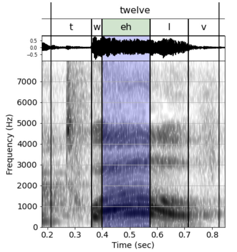
Plotting textgrid information with a spectrogram.
The second example shows that plot_tier() can be used to add lables directly to a spectrogram (or any other matplotlib axes).
phon.sgram(y, fs, cmap='Purples')
phon.plot_tier(wddf, vertical_place = 0.75)
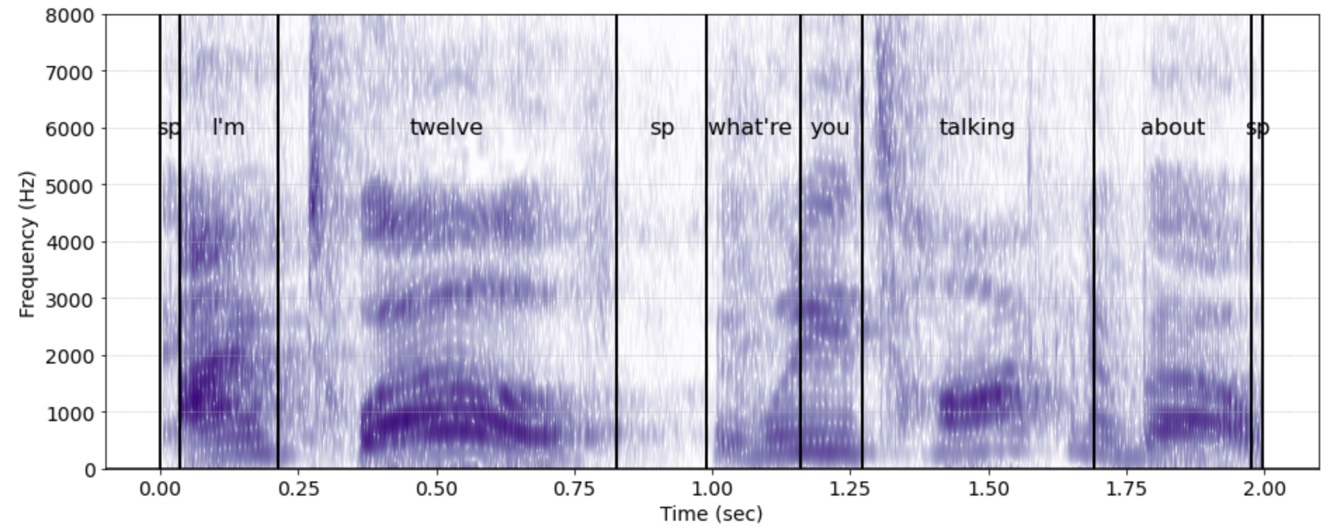
Adding textgrid labels to a spectrogram.
- phonlab.test_signal(type='sine', fs=10000, dur=0.5, freq=500, amp=1)[source]
Generate audio test signals of various types.
- Parameters:
type (string, default="sine") –
The type of waveform to be generated. May be one of:
”sine”,
”sawtooth”,
”triangle”,
”square”, or
”impulse”.
fs (integer, default = 10000) – The sampling rate of the returned audio test signal.
dur (float, default = 0.5) – The duration (in seconds) of the returned audio test signal
freq (numeric, default = 500) – The frequency (in Hz) of the returned audio test signal.
amp (float, default = 1.0) – The amplitude of the returned signal, ranging from 0 (silence) to 1 (maximum amplitude)
- Returns:
out – a one-dimensional numpy array of length dur * fs
- Return type:
ndarry
- Raises:
ValueError: – if the type parameter is not one of the allowed types.
import matplotlib.pyplot as plt

x = phon.test_signal('sawtooth',dur=1,freq=1000,amp=0.5)
plt.plot(x[0:50])
- phonlab.smoothn(y, isrobust=False, s=None, W=None, MaxIter=100, TolZ=0.001, z0=None, nS0=10, weightstr='bisquare', axis=None, sd=None, verbose=False)[source]
Robust spline smoothing for 1-D to N-D data. Damien Garcia
smoothn provides a fast, automatized and robust discretized smoothing spline for data of any dimension.
- Parameters:
y (numeric or logical array) – A uniformly-sampled array of input data array to be smoothed. y can be any N-D noisy array (time series, images, 3D data,…). Non-finite data (NaN or Inf) are treated as missing values.
isrobust (logical, default = False) – Use robust algorithm to minimize the influence of outlying data
s (numeric, default = None) – The larger s is, the smoother the output will be. If the smoothing parameter s is omitted it is automatically determined using the generalized cross-validation (GCV) method. If given it must be a real positive scalar value.
W (array, default=None) – an array of weights (real positive values) must be the same shape as the input array.
MaxIter (numeric, default =100) – The maximum number of iterations allowed to find the smooth. Iteration is used in the presence of weighted and/or missing values.
TolZ (float, default = 1e-3) – Termination tolerance on z. Iteration is used in the presence of weighted and/or missing values.
z0 (array, default = None) – An initial estimate of the smoothed array z
nS0 (numeric, default = 10) – Number of samples to use in estimating the smoothing parameter s
weightstr (string, default ='bisquare') – type of smoothing spline, options include “bisquare” (the default), “cauchy”, “talworth”
axis (tuple, default = None) – in multidimensional cases, the order in which the axes will be smoothed
sd (array, default=None) – an array used to compute the W array of weights with the formula W = 1./sd**2.
verbose (logical, default = False) – print some information or warnings
- Returns:
z (array of float) – The returned array, a smoothed version of the input array y
s (numeric) – The calculated value of s
exitflag (logical) – True means that smoothn converged False means that the maximum number of iterations was reached
References
Garcia (2010) Robust smoothing of gridded data in one and higher dimensions with missing values. Computational Statistics & Data Analysis 54 , 1187-1178. http://www.biomecardio.com/publis/csda10.pdf
Garcia (2011) A fast all-in-one method for automated post-processing of PIV data. Exp Fluids, 50 , 1247-1259. http://www.biomecardio.com/publis/expfluids11.pdf
Examples
x = np.linspace(0,100,2**5);
y = np.cos(x/10)+(x/50)**2 + np.random.random_sample(len(x))/2;
y[[14, 17, 20]] = [2, 2.5, 3];

z,s,e = phon.smoothn(y); # Regular smoothing
zr,sr,e = phon.smoothn(y,isrobust=True); # Robust smoothing

print(f'regular smoothing factor = {s:.3f}, robust smoothing factor = {sr:.3f}')

plt.subplot(121),
plt.plot(x,y,'r.')
plt.plot(x,z,'k')
plt.title("Smoothed")

plt.subplot(122)
plt.plot(x,y,'r.')
plt.plot(x,zr,'k')
plt.title("Robust Smoothing")
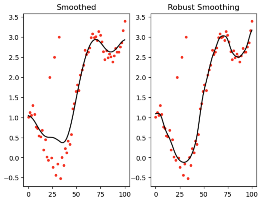
Comparing regular smoothing with robust smoothing with missing data and outliers in phon.smoothn()