Acoustic Phonetics

Spectrogram/waveform

phonlab.display_wave(x, fs, start=0, end=-1, ax=None, ylabel='Amplitude', font_size=14, **kwargs)

Use the matplotlib.pyplot.plot() function to plot an acoustic waveform or other time series.

Parameters:

• x (ndarray) – a one-dimensional array of audio samples, or other time series data.

• fs (numeric) – Sampling rate of the data in x

• start (float (default 0.0)) – start time of the plot’s x axis (in seconds)

• end (float (default -1)) – end time of the plot’s x axis (in seconds), default value of -1 means plot to the end of the data.

• ax (Matplotlib axes object (default None)) – by default (ax=None) a new matplotlib figure will be created.

• ylabel (string (default "Amplitude")) – The function is used to plot an audio waveform, so the default y-axis label is “Amplitude”. However, this function can be use to plot any time series.

• font_size (integer (default 14)) – Size of the text in the figure’s labels and tick labels.

• **kwargs (keyword arguments) – key word arguments will be passed to pyplot.plot()

Returns:

ax – The matplotlib axes

Return type:

Axes

Examples

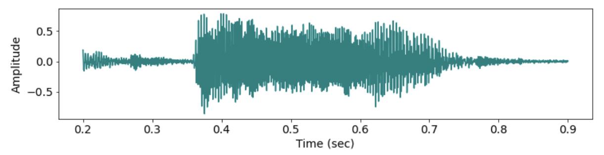
Plot a portion of the sound file from 0.2 to 0.9 seconds.

audio_dir = importlib.resources.files('phonlab') / 'data' / 'example_audio'
example_file = audio_dir / 'im_twelve.wav'

x,fs = phon.loadsig(example_file, chansel=[0])

ax = phon.display_wave(x,fs,0.2,0.9,color='teal')

phonlab.sgram(x, fs, start=0, end=-1, tf=8000, band='wb', preemph=0.94, font_size=14, min_prop=0.55, save_name='', slice_time=-1, cmap='Greys', resize=True, ax=None)

Make pretty good looking spectrograms

• This function calls scipy.signal.spectrogram to calculate a magnitude spectrogram, which is then transformed to decibels, and passed to plt.imshow for plotting.

• It mainly is used to produce nice looking figures with features like readable time and frequency axes, scaling so that the time axis is 6.5 inches per second for spectrograms of less than 2 seconds.

• The function also returns arrays that you can use to create your own figures.

• The function uses one of two window lengths - 40 msec for narrow band spectrograms, or 8 msec for wideband spectrograms.

• One option is to add a “spectral slice” to the display - the amplitude/frequency spectrum at a particular point in time.

Parameters:

• x (ndarray) – a one-dimensional array of audio samples.

• fs (numeric) – The sampling rate of the audio in x

• start (float, default = 0) – starting time (in seconds) of the waveform chunk to plot – default plot whole file

• end (float, default = -1) – ending time (in seconds) of the waveform chunk to plot (-1 means go to the end)

• tf (integer, default = 8000) – the top frequency (in Hz) to show in the spectrogram

• band (string, {'wb','nb'}) – effective filter bandwidth of the analysis filter (‘wb’ = 300 Hz, ‘nb’ = 45 Hz)

• preemph (float, default = 0.94) – add high frequency preemphasis before making the spectrogram, a value between 0 and 1

• font_size (integer, default = 14) – the font size to use for the axis labels and tick labels.

• min_prop (float, default = 0.2) – set the ‘floor’ of the gray scale. The default value specifies that the floor will be at 55% of the range between min and max amplitudes.

• save_name (Path, default = '') – name of a file to save the figure pyplot.savefig(), by default no file is saved.

• slice_time (float, default = -1) – location (in seconds) of an optional spectral slice.

• resize (boolean, default = True) – if a matplotlib axes object is passed in (the ax parameter), resize it to classical spectrogram dimensions.

• ax (a matplotlib axes object, default = None) – the user may provide a matplotlib object to which the spectrogram will be plotted.

• cmap (string, default = "Grays") – name of a matplotlib colormap for the spectrogram

Returns:

• ax (a matplotlib axes object) – The plot axes is returned

• f (ndarray) – Array of sample frequencies.

• t (ndarray) – Array of segment times.

• Sxx (ndarray) – Spectrogram of the audio. By default, the last axis of Sxx corresponds to the segment times. It is the magnitude spectrum on the decibel scale, so 20 * log10(Sxx) of the spectrogram returned by scipy.signal.spectrogram.

Examples

Plot a spectrogram of a portion of the sound file from 1.5 to 2 seconds. Then add a vertical red line at time 1.71

import matplotlib.pyplot as plt

audio_dir = importlib.resources.files('phonlab') / 'data' / 'example_audio'
example_file = audio_dir / 'sf3_cln.wav'

x,fs = phon.loadsig(example_file,chansel=[0])
phon.sgram(x,fs,start=1.5, end=2.0)
plt.axvline(1.71,color="red")

Marking the burst found by phon.burst()

Read a file into an array x, track the formant frequencies in the file, use them to produce sine wave speech, and then plot a spectrogram of the resulting signal.

example_file = importlib.resources.files('phonlab') / 'data' / 'example_audio' / 'sf3_cln.wav'

x,fs = phon.loadsig(example_file, chansel=[0])
fmtsdf = phon.track_formants(x,fs)    # track the formants
x2,fs2 = phon.sine_synth(fmtsdf)     # use the formants to produce sinewave synthesis
ax1,f,t,Sxx = phon.sgram(x2,fs2, band="nb", preemph=0)  # plot a spectrogram of it

Showing the spectrogram of sine-wave synthesis.

phonlab.compute_sgram(x, fs, w, s=0.001, order=13)

Compute a spectrogram from input waveform array of samples.

Parameters:

• x (ndarray) – array of audio samples

• fs (integer) – The sampling frequency of the audio samples in x

• w (float) – Length in seconds of the analysis window. For an effective filter bandwidth of 300 Hz use w = 0.008, and for an effective filter bandwidth of 45 Hz use w = 0.04.

• s (float, default=0.001) – The time (in seconds) between adjacent spectra in the spectrogram.

• order (integer, default = 13) – This parameter determines the number of points in the FFT analysis that produces the spectrogram. The number of points will be a power of 2 (2**order) and should be larder than the number of points in the analysis window (which is w*fs).

Returns:

• t (ndarray) – Array of segment times.

• f (ndarray) – Array of sample frequencies.

• Sxx (ndarray) – Spectrogram of the audio. By default, the last axis of Sxx corresponds to the segment times. It is the magnitude spectrum on the decibel scale, so 20 * log10(Sxx) of the spectrogram returned by scipy.signal.spectrogram.

phonlab.cepstral_smooth(x, fs, tf=5000, s=0.005, l=0.04, preemphasis=0.0, lift=0.003)

Smooth spectra by cepstral ‘liftering’ to remove the periodic source, leaving only the overall spectral envelope shape. The implementation here borrows heavily from Seonju Kim’s repository (https://github.com/hwang9u/pyceps).

Parameters:

• x (ndarray) – A one-dimensional array of audio samples

• fs (int) – Sampling rate of x

• tf (int, default = 5000) – The top frequency (in Hz) of the smoothed spectrum. The audio will be resampled to the sampling rate tf * 2.

• s (float, default = 0.005) – Step size, of hops between analysis windows. The default is 5 milliseconds.

• l (float, default = 0.04) – Length of analysis windows. The default is 40 milliseconds. The actual size of the analysis windows will be the smallest power of 2 that is greater than or equal to this length in samples.

• lift (float, default = 0.003) – The filtering coefficient (in seconds). Compenents that have a period longer than the lift value will be removed from the signal. The default value of 3 ms means that cepstral components lower than 333Hz will be removed. Smaller values of this parameter lead to more smoothing, and larger values lead to less spectral smoothing.

Returns:

• sec (ndarray) – A one dimensional numpy array with frame time points (in seconds)

• freqE (ndarray) – A one dimensional numpy array with frequency values (in Hz) for the smoothed spectral envelope, Exx.

• Exx (ndarray) – A two dimensional numpy array with cepstrally smoothed spectral magnitudes at these timepoints and frequencies. The spectrum at time point i is found at Exx[:,i].

• freqS (ndarray) – The frequency axis for the raw spectral array, Sxx.

• Sxx (nd array) – A two dimensional numpy array with raw spectral magnitudes, before smoothing. A narrow band spectrogram.

• quef (nd array) – A one dimensional numpy array with quefrency values (in ms) corresponding to axis 1 of the cepstra array, Cxx.

• Cxx (nd array) – A two dimensional numpy array of cepstra at the time points in sec.

References

2. 16. Bogert, M. J. R. Healy, and J. W. Tukey, (1963) The Quefrency Alanysis [sic] of Time Series for Echoes: Cepstrum, Pseudo Autocovariance, Cross-Cepstrum and Saphe Cracking, `Proceedings of the Symposium on Time Series Analysis (M. Rosenblatt, Ed) Chapter 15, 209-243. New York: Wiley.

import matplotlib.pyplot as plt

audio_dir = importlib.resources.files('phonlab') / 'data' / 'example_audio'
example_file = audio_dir / 'sf3_cln.wav'

x,fs = phon.loadsig(example_file,chansel=[0])

freq, ts, Exx, Sxx, quef, Cxx = phon.cepstral_smooth(x, fs, lift=0.0022)

# ------ plot spectra at a particular time point -------

slice_time = 1.4
i = np.argmin(np.abs(ts-slice_time))  # find the index of the spectral slice

plt.plot(freq,Exx[:,i], color='blue')
plt.plot(freq1,Sxx[:,i],alpha=0.2,color='gray')

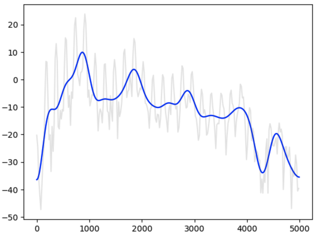
A ceptrally smoothed spectrum taken at time 1.4 in file sf3_cln.wav, in comparison with the unsmoothed FFT spectrum.

Amplitude Contour

phonlab.amplitude_envelope(x, fs, bounds=[], target_fs=22050, cutoff=30, order=2)

Get the amplitude envelope of an audio signal.

This routine rectifies the audio signal and then low pass filters it. This is different from calculating an RMS amplitude contour because it gives an amplitude measurement at each point in the audio rather than measuring amplitude in discrete windows. The filter is scipy.signal.sosfiltfilt()- a very stable filter that introduces no phase shift in the ouput waveform.

If bounds is supplied (eg. bounds = [100,2600]) then a bandpass filter with the low and high frequency edges specified in bounds will be applied.

Parameters:

• x (ndarray) – A 1-D array of audio samples

• fs (int) – the sampling frequency of the audio in x (in Hz)

• bounds (list, default = []) – a list (length 2) with the low and high edges of a bandpass filter. By default the function calculates the amplitude envelope for the full band from 0Hz to 11025 Hz (or whatever is the Nyquist frequency (1/2 of the target sampling rate).

• target_fs (int, default = 22050) – the desired sampling frequency of the output array

• cutoff (float, default = 30) – cutoff freq. for the low-pass envelope filter.

• order (int, default = 2) – order of the low-pass envelope filter

Returns:

• y (ndarray) – an array with the amplitude envelope, the array has the same number of samples as x

• fs (int) – the sampling frequency of the audio in y

Example

This example shows the use of phon.amplitude_envelope to calculate the amplitude contour in two frequency bands, and then the difference between them. This plot of the difference in the balance of energy between high and low frequency interestingly seems to segment the audio into vocalic and non-vocalic regions.

x,fs = phon.loadsig(example_file,chansel=[0])
hband, fs = phon.amplitude_envelope(x,fs,bounds=[3000,8000])
lband, fs = phon.amplitude_envelope(x,fs,bounds=[120,3000])
diff = lband-hband

time_axis = np.arange(len(diff))/fs
ax1,f,t,Sxx = phon.sgram(x,fs)  # plot the spectrogram
ax2 = ax1.twinx()
ax2.plot(time_axis,diff, color = "red")  # add scaled diff function
ax2.axhline(0)

Plotting the difference between the amplitude envelope in the low frequencies [120,3000] versus the amplitude envelope in high frequencies [3000,8000].

phonlab.get_rms(y, fs, s=0.005, l=0.04, scale=False)

Measure the time-varying root mean square (RMS) amplitude of the signal in y.

Parameters:

• y (ndarray) – A one-dimensional array of audio samples

• fs (int) – Sampling rate of x

• scale (boolean, default = False) – optionally scale the rms amplitude to maximum peak.

Returns:

df – There are two columns in the returned frame - sec, rms.

Return type:

pandas DataFrame

phonlab.intensity_to_df(obj, ts=None, interpolation='CUBIC', tcol='sec')

Return intensity values from a Praat Intensity object as a dataframe.

Parameters:

• obj (Praat Intensity obj) – An Intensity object produced by parselmouth.Sound(‘wavefile.wav’).to_intensity().

• ts (DataFrame, Iterable of floats, or None (default)) – If None (default), then the Intensity object’s ts times are used to query for intensity measurements. These are the centers of the analysis frames. The Intensity object’s values can also be queried at specific times by providing ts as an Iterable of floats, such as a numpy array or Python list. If ts is a dataframe, the column labelled by the tcol parameter is used for the time values and the intensity measures are concatenated to the dataframe.

• interpolation (str 'CUBIC' (default), 'NEAREST', 'LINEAR', 'SINC70', 'SINC700') – The type of interpolation to use when returning values. Lower case versions of the units are allowed. See Praat’s Intensity.cpp and Vector_enums.h files for defined values.

• tcol (str (default 'sec') or None) – The label of the time column in the output dataframe, ‘sec’ by default. If None, no time column is added to the dataframe.

Returns:

The output dataframe contains a column of intensity measurements labelled spl. The time column is labelled by the value of tcol (default ‘sec’), or omitted if tcol is None. If ts is a dataframe, the output is a concatenation of the input dataframe and the intensity measures.

Return type:

DataFrame

Examples

snd = parselmouth.Sound(mywav)
intens = snd.to_intensity()

spldf = phon.intensity_to_df(intens)  # Get dataframe of SPL.

## Now you can use all of the Pandas functions with your Praat data

spldf.to_csv('intensity.csv', sep='    ', header=True, index=False)
splddf.to_pickle('intensity.zip')

Formant Tracking

phonlab.track_formants(x, fs, method='lpc', preemphasis=1.0, f0_range=[63, 400], speaker=0, order=-1, quiet=False)

Computes the vowel formant values in audio of speech.

The function uses either LPC analysis or the IFC method to calculate vowel formants (the resonant frequencies of the vocal tract) and then returns a dataframe of measurements (formants, f0, voicing, and amplitude) at 10ms intervals for the duration of sound.

The IFC option uses the Watenabe/Ueda Inverse Filter Control method of vowel formant tracking (Watenabe, 2001; Ueda et al., 2007). This method can be quite a bit more accurate than LPC, but is also substantially slower. In addition to calculating formants, the function uses the estimated formant frequencies to inverse filter the waveform and then calculate f0 (voice pitch) from the quasi glottal waveform using autocorrelation. The peak autocorrelation values are normalized and returned as a voicing score between 0 and 1. Finally, the RMS amplitude of the preemphasised waveform is also returned.

The LPC option uses the Librosa implemenation of Burg’s (1975) autocorrelation method for linear predictive coding and then polynomial root solving to find the vowel formant frequencies. The function also uses the LPC coefficients to inverse filter the waveform and then calculate f0 (voice pitch) from the quasi glottal waveform using autocorrelation. The peak autocorrelation value of each frame is also returned. Finally, the RMS amplitude of the waveform is also returned.

Parameters:

• x (array) – a one-dimensional array of audio samples

• fs (int) – the sampling rate of the audio in x

• preemphasis (float, default = 1.0) – factor of a preemphasis factor (0-1).

• f0_range (list, default = [63,400]) – the lowest and highest values to consider in pitch tracking.

• method (string, default = "lpc") –

  a string indicating which formant tracking method to use.

  • lpc - Linear predictive coding (the default value)

  • ifc - Inverse filter control

  • ifc_old - a slower direct python implementation of Ueda et al.’s code

  • ifc_fast - a much faster but less accurate approach to IFC

• speaker (int, default = 0) –

  set formant expectations for IFC. This parameter is only used in IFC analysis.

  • 0 = long vocal tract, male speaker

  • 1 = medium, female speaker

  • 2 = small, a child.

• order (int, default = -1) – the default value, -1 tries several values of lpc_order and determines the best value for this audio file. You can also specify the order by setting this parameter to a positive integer (12 or 14 for a male speaker, 10 or 12 for a female speaker, 8 or 10 for a child). This parameter is only used in LPC analysis.

• quiet (boolean, default = False) – False means print progress or warning messages

Returns:

df – a pandas dataframe with formant, f0, amplitude, and voicing score measurements at 0.01 sec intervals.

Return type:

dataframe

Note

The columns in the output dataframe are:

• sec - midpoint time of the frame

• rms - the rms amplitude

• F1-4 - the lowest four vowel ‘formants’ - vocal tract resonances.

• f0 - the fundamental frequency of voicing

• c - the autocorrelation value, higher indicates stronger evidence of voicing

References

10. 16. Burg (1975) Maximum entropy spectral analysis, Ph.D. dissertation, Dep. Geophys., Stanford Univ., Stanford, CA.

1. Watenabe (2001) Formant estimation method using inverse-filter control. IEEE Trans. Speech Audio Processing, 9, 317-326.

25. Ueda, T. Hamakawa, T. Sakata, S. Hario, & A. Watanabe (2007) A real-time formant tracker based on the inverse filter control method. Acoustical Science and Technology, 28 (4), 271–274. https://doi.org/10.1250/ast.28.271

Examples

Use Inverse Filter Control to track formants in a file

df = phon.track_formants(x,fs,method='ifc',speaker=1)

The next example uses LPC analysis, which by default will try to pick the best lpc_order for the speaker. An array of samples is loaded by phon.loadsig() and then passed to phon.track_formants(). Then phon.sgram() plots the spectrogram of x, and the seaborn graphics package is used to add the formants to the spectrogram.

example_file = importlib.resources.files('phonlab') / 'data' / 'example_audio' / 'sf3_cln.wav'
x,fs = phon.loadsig(example_file, chansel=[0])
fmtsdf = phon.track_formants(x, fs)

ret = phon.sgram(x,fs, tf=6000, cmap="Reds")  # plot the spectrogram

dot_color = "dodgerblue"
sns.pointplot(fmtsdf,x='sec',y='F1',linestyle='none',native_scale=True,marker=".",color=dot_color)
sns.pointplot(fmtsdf,x='sec',y='F2',linestyle='none',native_scale=True,marker=".",color=dot_color)
sns.pointplot(fmtsdf,x='sec',y='F3',linestyle='none',native_scale=True,marker=".",color=dot_color)
sns.pointplot(fmtsdf,x='sec',y='F4',linestyle='none',native_scale=True,marker=".",color=dot_color)

fmtsdf.to_csv("sf3_cln.csv",index=False)

Plotting the formants found by track_formants(… method=’ifc’), on the spectrogram of the utterance.

phonlab.RLPC_formants(x, fs, tf=6000, preemphasis=0.94, order=-1, base='BIC', s=0.01, l=0.03, window=None, numiter=1, verbose=False)

An implementation of Lee’s (1988) method for Robust Linear Prediction Coding. The method computes the residual signal from a conventional LPC analysis and then uses it to down-weight samples that produce large prediction error. It is possible to iterate the residual reweighting process more than once, though not much improvement is gained after the first iteration. Formant frequencies are found from the LPC coefficients using polynomial root solving. A couple of functions called by RLPC_formants() are accelerated by the use of numba just in time (JIT) compilation into machine code. Therefore, the first call to RLPC_formants() will be slower (by about 10 ms) than subsequent calls.

Note that unlike other formant analysis functions, this one returns both a dataframe with analysis results and also a 2D matrix with time-varying LPC coefficients.

Parameters:

• x (ndarray) – a 1D array of audio samples

• fs (int) – the sampling rate of samples in x. This will be resampled to 12,000 Hz for analysis, so choose the order paramter with this in mind.

• tf (int (default = 6000)) – The top frequency of the analysis band. The input signal will be resampled to a rate of tf*2.

• preemphasis (float (default = 0.94)) – value of a high frequency preemphasis (spectral tilt) factor (0-1).

• order (int (default = -1)) – The LPC ‘order’ (i.e. the number of coefficients in the LPC filter. A value of -1 uses the function phon.choose_order() to determine the best value for this parameter.

• base (string (default = 'BIC')) – If order is -1, then use this base (‘BIC’ or ‘coef’) in phon.choose_order().

• s (float (default = 0.01)) – the interval (in seconds) between successive formant measurements.

• l (float (default = 0.05)) – duration (in seconds) of analysis frames

• window (string (default = 'cosine')) – The name of a window shape for scipy.signal.windows.get_window()

• numiter (integer (default = 1)) – Number of robust LPC iterations to perform. If this value is 0 the results of the conventional LPC analysis are returned with no robust recalculation of the linear prediction.

• verbose (boolean (default = False)) – Print diagnostic messages

Returns:

• df - a pandas dataframe with columns as described in the note below.

• A - a two-dimensional numpy matrix with the LPC coefficients for each analysis frame.

Note

The columns in the output dataframe are:

• sec - midpoint time of the frame

• gain - the LPC gain (variance of the residual) for each frame.

• F1-4 - the lowest four vowel ‘formants’ - vocal tract resonances.

• BW1-4 - bandwidths of the vowel formants

References

C.H. Lee (1988) On robust prediction of speech. IEEE Transactions on Acoustics, Speech and Signal Processing, 36,5: 642-650.

phonlab.TVLP_formants(x, fs, tf=6000, order=-1, frame_duration_sec=0.1, q=3, norm='l2', qcp=True, step=0.01, nformants=4, f0median=200, max_bandwidth=800, use_parallel=False, verbose=False)

This formant tracking function implements the time-varying, pitch synchronous, method that was described by Gowda et al. (2020). The most important innovation of this method is that it smooths the Linear Prediction coefficients over time, providing a continuity constraint at the level of the LP coefficients. The second most important method is that (like Robust LPC) the method can optionally weight the audio samples pitch synchronously so the LP coefficients are caluculated from the glottal closed phase where the assumptions of LPC analysis are better met. The third innovation, which also seems to be both the most computationally costly and least important for good formant tracking, is that the LP coefficients can be calculated minimizing the L1 norm (city-block) norm rather than the default L2 norm (Euclidian distance). The L1 norm is 10 times slower than the L2 norm and results in almost no change in the derived formant frequencies.

This Python implementation is a translation (done with extensive help from the AI model Claude) of Gowda’s ftrack matlab code. It uses numba for just-in-time (JIT) compilation of machine code, and parallelization of some loops which dramatically increases the speed of processing. However, the first call to the function includes the compilation of the JIT code (on a typical laptop this can be 10 seconds!). Subsequent calls to TVLP_formants() will use the compiled JIT code and be much faster than the first call. However, in some situations you may want to separate the compilation from the first call to TVLP_formants(). Therefore a helper function tvlp_warmup_numba() is provided. The helper function can be called at the beginning of a session to compile the JIT code, and then all subsequent calls to TVLP_formants() will be accelerated by the numba functions.

Parameters:

• x (array_like) – a one-dimensional array of audio samples

• fs (int) – Sampling frequency of x in Hz

• tf (int, default = 6000) – Top frequency. The signal will be resampled to tf*2.

• order (int, default = 10) – The number of LPC coefficients to use – the ‘order’ of the LPC filter. If this parameter is -1 then we will use phon.choose_order(base=’BIC’) to determine the best value for this parameter.

• frame_duration_sec (float, default 0.1 = 100ms) – Duration of each frame in seconds. Gowda et al.’s tests found that 100ms provides the most accurate formant measurements.

• q (int, default = 3) – Time-varying polynomial order

• norm (str, default = 'l2') – Choose whether to minimize the ‘l1’ or ‘l2’ norm in finding the LP and polynomial coefficients. The L1 norm requires an iterative reweighting algorithm which is much slower than minimizing the L2 norm.

• qcp (bool, default = True) – Choose whether or not to do a pitch synchronous analysis, limiting the estimation function to the glottal closed phase (the Quasi-Closed-Phase). If True the analysis will be pitch synchronous.

• step (float, default = 0.01) – Time interval between formant measurements in seconds. Formants are taken from the middle of each interval

• nformants (int, default=3) – Number of formants to extract

• f0median (float, default=200.0) – This is an estimate of the median F0 value to expect in the signal being analyzed. This parameter is used in the pitch synchronous method (i.e. when qcp is True) to guide the algorithm’s expectation for finding glottal closure intervals. It is important to get this approximately correct.

• max_bandwidth (float, default=800) – Maximum formant bandwidth in Hz, formants with bandwidth greater than this are rejected.

• use_parallel (bool, default=True) – Try to use parallel processing for formant extraction. Note: Usually doesn’t work in Jupyter notebooks, set to False for notebooks

• verbose (bool, default=False) – Print progress

Returns:

df – See the note. The number of formant columns depends on the nformants parameter.

Return type:

a Pandas DataFrame

Note

The columns in the output dataframe are:

• sec - midpoint time of the frame

• F1-4 - the lowest four vowel ‘formants’ - vocal tract resonances.

• BW1-4 - bandwidths of the vowel formants

References

4. Gowda, R. Kadiri, B. Story, P. Alku (2020) Time-varying quasi-closed-phase analysis for accurate formant tracking in speech signals. in IEEE/ACM Transactions on Audio, Speech, and Language Processing, vol. 28, pp. 1901-1914, doi: 10.1109/TASLP.2020.3000037.

phonlab.tvlp_warmup_numba(verbose=True)

Pre-compile Numba functions for TVLP_formants() with minimal data.

Parameters:

verbose (string, default='True') –

phonlab.DPPT_formants(x, fs, pre=0, l=0.03, s=0.01, deltaF=1100, n=6)

Bozkurt et al.’s (2004) Differential-Phase Peak Tracking (DPPT) method of vowel formant tracking is implemented in this function. The implementation here is a translation and interpretation of the matlab routine formant_CGDZP() written by Bozkurt and Drugman and published in the Covarep repository.

This algorithm tracks formants as peaks in the smoothed spectrum, therefore tends to be more likely than the LPC or IFC methods to track the harmonics of the voice fundamental frequency when pitch is high, and to report a single peak when formants have similar frequencies - reporting the same formant frequency for the close formants, such as when F1 and F2 are close in [u] or F2 and F3 are close in [i].

It may be that measuring the peaks in a smoothed spectrum is a more perceptually valid representation of vowel acoustics than a model that focusses on determining the resonances of the vocal tract (see Chistovich & Lublinskaya, 1979). Thus, it is appropriate to consider the formant frequencies reported by this DPPT algorithm to be perceptual formants.

Parameters:

• x (array) – a one-dimensional array of audio samples

• fs (int) – the sampling rate of the audio in x

• deltaF (int, default = 1100) – The expected average interval between formants, used to sort peaks into formant numbers.

• preemphasis (float, default = 0) – value of the preemphasis factor (0-1). It almost never helps to change this.

• l (float, default = 0.03) – Length of the pitch analysis window in seconds. The default is 30 milliseconds.

• s (float, default = 0.01) – “Hop” interval between successive analysis windows. The default is 10 milliseconds

• n (int, default = 6) – The required width of a peak, in terms of the number of steps in the spectrum. The default as in Bozkurt et al. is about 80 Hz wide.

Returns:

df – a pandas dataframe with formant measurements at 10 ms intervals (by default).

Return type:

dataframe

Note

The columns in the output dataframe are:

• sec - measurement time

• F1-4 - the lowest four vowel formants - peaks in the smoothed spectrum.

References

2. Bozkurt, B. Doval, C.D. Alessandro, T. Dutoit (2004) Improved differential phase spectrum processing for formant tracking. InterSpeech ICSLP, 8th International Conference on Spoken Language Processing, Jeju Island, Korea.

12. 1. Chistovich, V.V Lublinskaya (1979) The ‘center of gravity’ effect in vowel spectra and critical distance between the formants: Psychoacoustical study of the perception of vowel-like stimuli. Hearing Research, 1, 185-195.

Examples

This code block shows a call to phon.track_formants_DPPT() and also shows a call to LPC formant tracking, the default method in phon.track_formants(), and uses phon.sgram, and seaborn pointplot() to plot the estimated formant frequences on the spectrogram.

example_file = importlib.resources.files('phonlab') / 'data/example_audio/sf3_cln.wav'
x,fs = phon.loadsig(example_file,chansel=[0])

ret = phon.sgram(x,fs, tf=6000, cmap="Reds")  # plot the spectrogram

dflpc = phon.track_formants(x,fs)

dot_color = 'dodgerblue'
sns.pointplot(dflpc,x='sec',y='F1',linestyle='none',native_scale=True,marker=".",color=dot_color)
sns.pointplot(dflpc,x='sec',y='F2',linestyle='none',native_scale=True,marker=".",color=dot_color)
sns.pointplot(dflpc,x='sec',y='F3',linestyle='none',native_scale=True,marker=".",color=dot_color)
sns.pointplot(dflpc,x='sec',y='F4',linestyle='none',native_scale=True,marker=".",color=dot_color)

df = phon.track_formants_DPPT(x,fs,deltaF=1100)

dot_color = "darkblue"
sns.pointplot(df,x='sec',y='F1',linestyle='none',native_scale=True,marker=".",color=dot_color)
sns.pointplot(df,x='sec',y='F2',linestyle='none',native_scale=True,marker=".",color=dot_color)
sns.pointplot(df,x='sec',y='F3',linestyle='none',native_scale=True,marker="x",color=dot_color)
sns.pointplot(df,x='sec',y='F4',linestyle='none',native_scale=True,marker=".",color=dot_color)

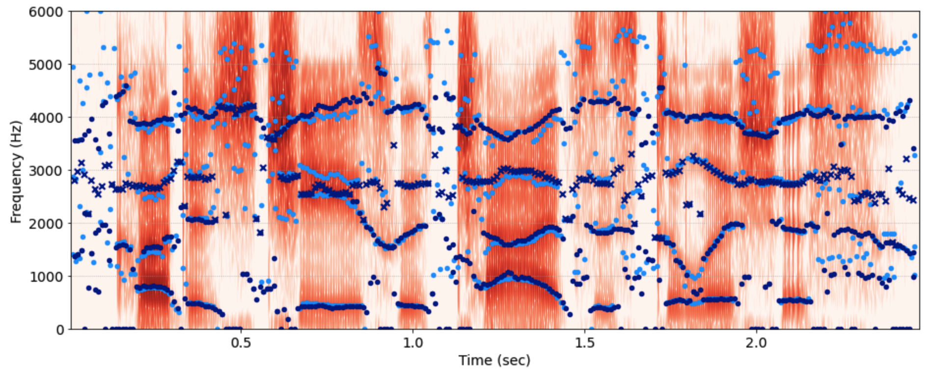
Plotting the formants found by track_formants() (light blue dots) and those found by track_formants_DPPT() (dark blue dots) on the spectrogram of the utterance.

phonlab.formant_to_df(obj, num, ts=None, unit='HERTZ', include_bw=False, tcol='sec')

Return formant values from a Praat Formant object as a dataframe.

See the examples for calls using the Parselmouth bindings to Praat.

Parameters:

• obj (Praat formant obj) – The input Formant object, which is produced by a call to Praat with parselmouth.Sound(‘wavefile.wav’).to_formant_burg()

• num (int or list of int) – The formants from which values will be returned. If num is int type the values of the first num formants are returned. If num is a list of numbers then the formants in the list are returned.

• ts (DataFrame, Iterable of floats, or None (default)) – If None (default), then the Formant object’s ts times are used to query for formant measurements. These are the centers of the analysis frames. The Formant object’s values can also be queried at specific times by providing an Iterable of floats, such as a numpy array or Python list.

• unit (str, 'HERTZ' (default) or 'BARK') – The unit in which formant values are returned. Lower case versions of the units are allowed. See Praat’s Formant_enums.h file for defined values.

• include_bw (boolean, default False) – If True, bandwidth values for each formant returned are also included.

• tcol (str (default 'sec') or None) – The label of the time column in the output dataframe, ‘sec’ by default. If None, no time column is added to the dataframe.

Returns:

The output dataframe contains columns of times and formant measurements. The formant columns are labelled FN, where N is an integer. The time column is labelled by the value of tcol (default ‘sec’), or omitted if tcol is None. If include_bw is True then bandwidth columns labelled bwN that correspond to FN columns are also returned. If ts is a dataframe, the output is a concatenation of the input dataframe and the formant/bandwidth measures.

Return type:

DataFrame

Examples

snd = parselmouth.Sound(mywav).extract_left_channel()

maxf = 5000       # a vocal tract length parameter, maximum frequency of F4
fmnt = snd.to_formant_burg(maximum_formant=maxf)

f12df = phon.formant_to_df(fmnt, 4, include_bw=True)  # convert praat to dataframe

f2df = phon.formant_to_df(fmnt, [2], unit='bark')  # or just the second formant

f1df.to_csv('formants.csv', sep='      ', header=True, index=False) # save to csv
f1df.to_pickle('formants.zip')

phonlab.choose_order(x, fs, l=0.03, base='BIC', verbose=False)

The most impactful parameter in LPC formant tracking is the ‘order’,the number of LPC coefficients to use in calculating a fit to the spectrum. Many authors propose a rule of thumb having to do with the expected number of formants in the analyzed frequency range: namely that the order should 2*nf + 2 (two times the number of formants expected in the frequency range of the analysis [0, fs/2] plus 2).

This function instead tests a number of different values of LPC order and returns the order value that results in the lowest Bayesian Information Criterion (BIC). The proceedure is to (1) select a 30 ms (by default) frame of audio waveform samples around the time of the peak amplitude in the band-limited (120Hz to 3000Hz) amplitude envelope of x, (2) then calculate LPC coeffients and BIC for each of several lpc orders (from fs/1000 - 2 to fs/1000 + 6) for that frame, and then (3) return the best order based on how well the LPC analysis fits the audio spectrum.

If base is ‘BIC’, the function returns the lpc order that produces the lowest Bayesian Information Criterion of the LPC residual as a function of the number of LPC coefficients.

If ‘base’ is ‘coef’, the function returns the lpc order that maximizes the first LPC coefficient, as a measure of the LPC filter gain.

Parameters:

• x (ndarray) – a one-dimensional numpy arry with audio waveform samples

• fs (int) – the sampling frequency of x

• l (float (default=0.03)) – the duration (in seconds) of the analysis frame (default=0.03)

• base (string (default = "BIC")) – see above.

• verbose (boolean (default = False)) – if True, print messages about the operation of the function

Returns:

• lpc_order (int) – the best fitting order term for LPC analysis

• time (float) – the time (in seconds) of the analysis frame.

phonlab.get_deltaF(df, return_value='deltaF')

Calcuate the delta F vocal tract length factor from formant values in a dataframe df. The estimate is more stable when the dataframe contains a representative set of vowels spoken by the talker (see Johnson, 2020).

Parameters:

• df (DataFrame) – The input dataframe must contain columns for F1, F2, F3, and F4. See phon.track_formants()

• return_value (string, default = "deltaF") – By default the deltaF normalization factor is returned. Normalized formant values are Fn/deltaF. If you specify return_value = “VTL”, then the function will return the estimated vocal tract length as VTL=35300/(2*∆F), where 35300 is the speed of sound (cm/sec) in warm air.

Returns:

deltaF or VTL – the quantity returned depends on the parameter return_value.

Return type:

numeric

References

11. Johnson (2020) The Delta F method of vocal tract length normalization for vowels. Laboratory Phonology, 11(1), 10. DOI: http://doi.org/10.5334/labphon.196

Example

fmtsdf = phon.track_formants(x,fs)
VTL = phon.get_deltaf(fmtsdf,return_value='VTL')

phonlab.deltaF_norm(df, column=None, deltaF=None)

Perform vocal tract length normalization (deltaF normalization) for each speaker indicated by a ‘groupby’ variable in a dataframe of vowel formant measurements. The estimate is more stable when the dataframe contains a representative set of vowels spoken by the talker (see Johnson, 2020).

Parameters:

• df (DataFrame) – The input dataframe must contain columns for F1, F2, F3, and F4. See phon.track_formants(). If multiple dataframes from different talkers have been combined into a large multitalker data frame, then there should be a column identifying the speaker for each row, and the name of this column should be passed as the groupby input variable.

• groupby (string, default=None) – If df contains data from more than one talker, the talker identity should be indicated in a column and the name of that column passed in this input variable.

• deltaF (numeric or None, default=None) – Supply a value of deltaF to be used for the normalization. By default the deltaF normalization factor is computed by the function phon.get_deltaF() over the data in the DataFrame you pass in.

Note

Nothing is returned by this function. The input dataframe is modified in place with the addition of five new columns – normalized values of the formants ‘F1/∆F’, ‘F2/∆F’, ‘F3/∆F’, ‘F4/∆F’, and the ‘deltaF’ factor used for normalization.

References

11. Johnson (2020) The Delta F method of vocal tract length normalization for vowels. Laboratory Phonology, 11(1), 10. DOI: http://doi.org/10.5334/labphon.196

Example

fmtsdf = phon.track_formants(x,fs)
phon.deltaF_norm(fmtsdf)  # add normalized formant columns
fmtsdf.head()  # now there are five new columns in the dataframe

phonlab.resize_vt(df, deltaf)

Compute new vowel formant values, from normalized values, as produced by the phonlab.deltaF_norm() function, using a new target deltaF value to produce a new non-normalized set of vowel formants. This simulates changing the length of the speaker’s vocal tract.

Parameters:

• df (DataFrame) – The input dataframe must contain columns labeled ‘F1/∆F’, ‘F2/∆F’, ‘F3/∆F’, and ‘F4/∆F’. See phon.track_formants() and phon.deltaF_norm(). These should be data from a single speaker.

• deltaf (float) – The new deltaF value that will be used to calcuate the non-normalized values from the Fx/∆F normalized values.

Returns:

df – New columns called ‘new_F1’, ‘new_F2’, etc. are added to the input DataFrame.

Return type:

DataFrame

Pitch Tracking

phonlab.get_f0(y, fs, f0_range=[63, 400], s=0.005)

Track the fundamental frequency of voicing (f0), using autocorrelation

This function implements the autocorrelation method described in Boersma (1993). where the autocorrelation function is normalized by the autocorrelation of the analysis window. The raw best fit frame-by-frame values are returned – that is, this function does not follow Boersma (1993) in using the Viterbi algorithm to choose the optimal path among f0 candidates.

The Harmonics-to-Noise ratio (HNR) in each frame is estimated from the peak of the autocorreation function (c) as 10 * log10(c/(1-c)).

Probability of voicing is given from a logistic regression formula using rms and c to predict the voicing state as determined by EGG data using the function phonlab.egg_to_oq() over the 10 speakers in the ASC corpus of Mandarin speech. The prediction of the EGG voicing decision was about 86% correct.

Parameters:

• y (ndarray) – A one-dimensional array of audio samples

• fs (int) – Sampling rate of x

• f0_range (list of two integers, default = [63,400]) – The lowest and highest values to consider in pitch tracking.

• s (float, default = 0.005) – “Hop” interval between successive analysis windows. The default is 5 milliseconds

Returns:

df – measurements at 5 msec intervals.

Return type:

pandas DataFrame

Note

The columns in the returned dataframe are for each frame of audio:

• sec - time at the midpoint of each frame

• f0 - estimate of the fundamental frequency

• rms - peak normalized rms amplitude in the band from 0 to fs/2

• c - value of the peak autocorrelation found in the frame

• HNR - an estimate of the harmonics to noise ratio

• probv - probability of being voiced

• voiced - a boolean, true if probv > 0.5

References

16. Boersma (1993) Accurate short-term analysis of the fundamental frequency and the harmonics-to-noise ratio of a sampled sound. Institute of Phonetic Sciences, Amsterdam University, Proceedings. 17, 97-110.

Comparing the f0 found by phon.get_f0() plotted in blue, and the f0 values found by parselmouth to_Pitch(), plotted with chartreuse dots, and the f0 values found by get_f0_acd, plotted in orange. The traces are offset from each other by 10Hz so they can be seen.

phonlab.get_f0_shs(x, fs, f0_range=[50, 400], l=0.06, s=0.005, shr_threshold=0.3, target_time=None)

A pitch determination function implementing the subharmonic summation (SHS) algorithm proposed by Dik Hermes (1988), with a method of finding the relative amplitude of a subharmonic pitch (if there is evidence of a subharmonic) as suggested by Xuejing Sun (2002). The method is good at tracking pitch changes when the voice goes into creak, and is relatively insensitive to the setting of the f0_range parameter. If you find that there is pitch halving, try increasing the shr_threshold, and if you find pitch doubling try decreasing shr_threshold and/or the top end of the f0_range.

Parameters:

• x (ndarray) – A one-dimensional array of audio samples

• fs (int) – Sampling rate of x

• f0_range (an array of two numbers, default=[50,400]) – The expected range for f0. There is rarely any need to adjust the lower value.

• l (float, default = 0.06) – Length of analysis windows. The default is 60 milliseconds.

• s (float, default = 0.005) – Step size, of hops between analysis windows. The default is 5 milliseconds.

• shr_threshold (float, default = 0.3) – A value which determines how sensitive the algorithm is in deciding that a subharmonic component is present in the voicing spectrum.

• target_time (float, default = None) – If a time value (in seconds) is given, a diagnostic figure comparable to Sun’s Figure 1 will be produced for the frame at time target_time.

Returns:

df – measurements at (by default) 5 msec intervals.

Return type:

pandas DataFrame

Note

The columns in the returned dataframe are for each frame of audio:

• sec - time at the midpoint of each frame in seconds

• f0 - estimate of the fundamental frequency in Hz

• rms - rms amplitude in the frequency band from 0 to fs/2

• shr - The Subharmonic-to-harmonic Ratio. If the ratio is low the subharmonic energy is close to that of the harmonic.

References

4. Hermes (1988) Measurement of pitch by subharmonic summation. J. Acoust. Soc. Am., 83(1),257-264.

24. Sun (2002) Pitch determination and voice quality analysis using subharmonic-to-harmonic ratio. Proceedings of ICASSP2002 I-333 - I-336.

Example

example_file = importlib.resources.files('phonlab') / 'data/example_audio/sf3_cln.wav'
x,fs = phon.loadsig(example_file,chansel=[0])
ttime = 2.101

df = phon.get_f0_shs(x,fs, shr_threshold=0.2, target_time=2.1)

This example shows diagnostic plots from the get_f0_shs() function. The top left panel shows the spectrum at a particular time in the audio file on a log2 scale. The top right and bottom left panels show harmonic and subharmonic summation spectra which are used to produce the difference spectrum in the bottom right. The maximum of the difference spectra is taken as the pitch in this frame.

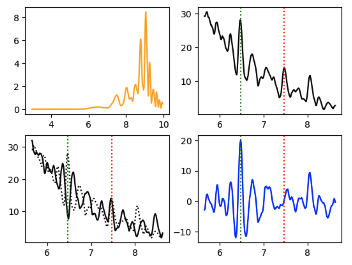
Diagnostic plots from shr_pitch().

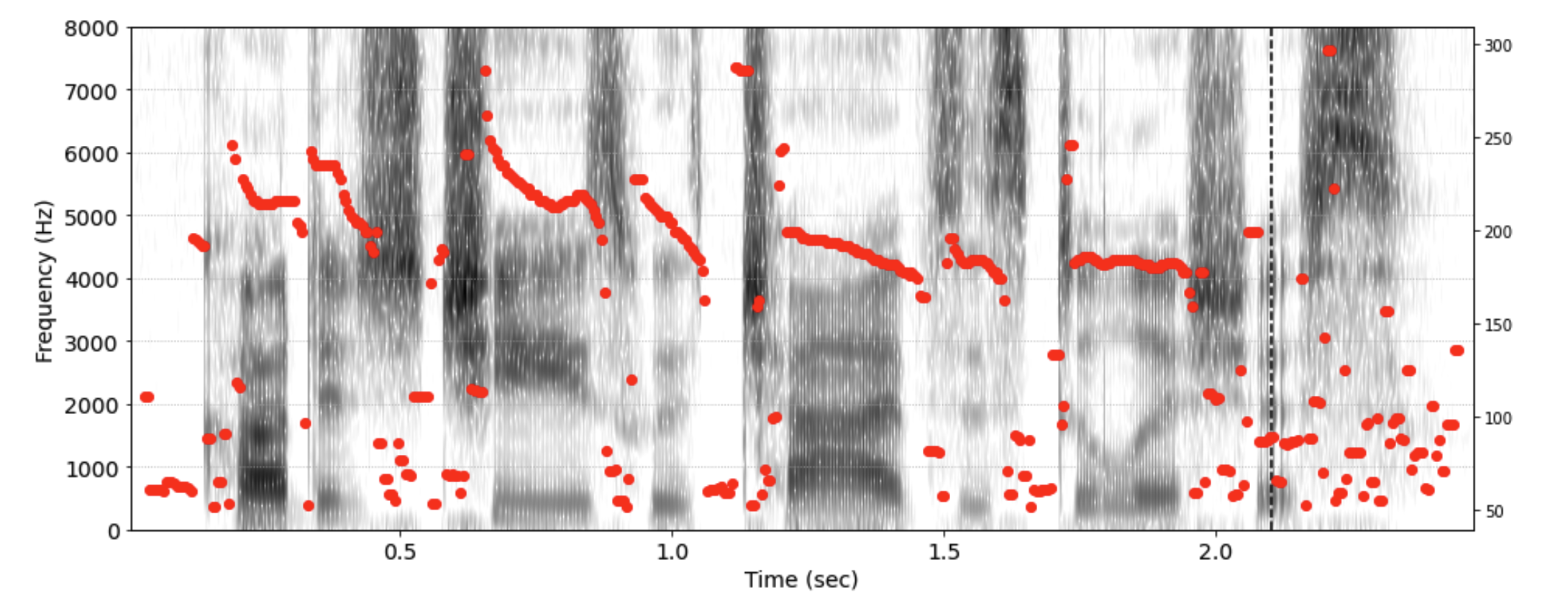
Pitch trace produced by get_f0_shs() function.

phonlab.get_f0_acd(y, fs, f0_range=[60, 400], l=0.05, s=0.005, prom=5, min_height=0.6, test_time=-1)

Track the fundamental frequency of voicing, using a frequency domain method.

This function implements the ‘approximate common denominator” algorithm proposed by Aliik, Mihkla and Ross (1984), which was an improvement on the method proposed by Duifuis, Willems and Sluyter (1982). The algorithm finds candidate harmonic peaks in the spectrum, and chooses a value of f0 that best predicts the harmonic pattern. One feature of this method is that it reports a voice quality measure (the difference in the amplitudes of harmonic 1 and harmonic 2).

Probability of voicing is given from a logistic regression formula using rms, the h2h1 ratio, and Duifuis et al.’s harmonicity criterion C to predict the voicing state as determined by EGG data using the function phonlab.egg_to_oq() over the 10 speakers in the ASC corpus of Mandarin speech. The prediction of the EGG voicing decision was about 86% correct. Aliik et al. (1984) used a cutoff of C < 3.5 as a voicing threshold.

Parameters:

• y (ndarray) – A one-dimensional array of audio samples

• fs (int) – the sampling rate of the audio in y.

• f0_range (a list of two integers, default=[60,400]) – The lowest and highest values to consider in pitch tracking. The algorithm is not particularly sensitive to this parameter, but it can be useful in avoiding pitch-halving or pitch-doubling.

• l (float, default = 0.05) – Length of the pitch analysis window in seconds. The default is 50 milliseconds.

• s (float, default = 0.005) – “Hop” interval between successive analysis windows. The default is 5 milliseconds

• prom (numeric, default = 5 dB) – In deciding whether a peak in the spectrum is a possible harmonic, this prominence value is passed to scipy.find_peaks(). A larger value means that the spectral peak must be more prominent to be considered as a possible harmonic peak, and thus the algorithm is less likely to report pitch values when the parameter is given a high value. In general, 20 is a high value, and 3 is low.

• min_height (numeric, default = 0.6) – As a proportion of the range between the lowest amplitude in the spectrum and the highest, only peaks above min_height will be considered to be harmonics. The value that is passed to find_peaks() is: amplitude_min + min_height*(amplitude_range).

Returns:

df – measurements at 5 msec intervals.

Return type:

pandas DataFrame

Note

The columns in the returned dataframe are for each frame of audio:

• sec - time at the midpoint of each frame

• f0 - estimate of the fundamental frequency

• rms - rms amplitude in a low frequency band from 0 to 1200 Hz

• h1h2 - the difference in the amplitudes of the first two harmonics (H1 - H2) in dB

• C - harmonicity criterion (lower values indicate stronger harmonic pattern)

• probv - estimated probability of voicing

• voiced - a boolean, true if probv>0.5

References

10. Allik, M. Mihkla, J. Ross (1984) Comment on “Measurement of pitch in speech: An implementation of Goldstein’s theory of pitch perception” [JASA 71, 1568 (1982)]. JASA 75(6), 1855-1857.

8. Duifhuis & L.F. Willems (1982) Measurement of pitch in speech: An implementation of Goldstein’s theory of pitch perception. JASA 71(6), 1568-1580.

Example

example_file = importlib.resources.files('phonlab') / 'data' / 'example_audio' / 'stereo.wav'

x,fs = phon.loadsig(example_file, chansel=[0])
f0df = phon.get_f0_acd(x,fs,prom=18)

snd = parselmouth.Sound(str(example_file)).extract_left_channel()  # create a Praat Sound object
pitch = snd.to_pitch()  # create a Praat pitch object
f0df2 = phon.pitch_to_df(pitch)  # convert it into a Pandas dataframe

ret = phon.sgram(x,fs,cmap='Grays') # draw a spectrogram of the sound

f0_range = [60,400]

ax1 = ret[0]  # get the plot axis
ax2 = ax1.twinx()  # and twin it for plotting f0
ax2.plot(f0df2.sec,f0df2.f0, color='chartreuse',marker="s",linestyle = "none")
ax2.plot(f0df.sec,f0df.f0, color='dodgerblue',marker="d",linestyle = "none")
ax2.set_ylim(f0_range)
ax2.set_ylabel("F0 (Hz)", size=14)
for item in ax2.get_yticklabels(): item.set_fontsize(14)

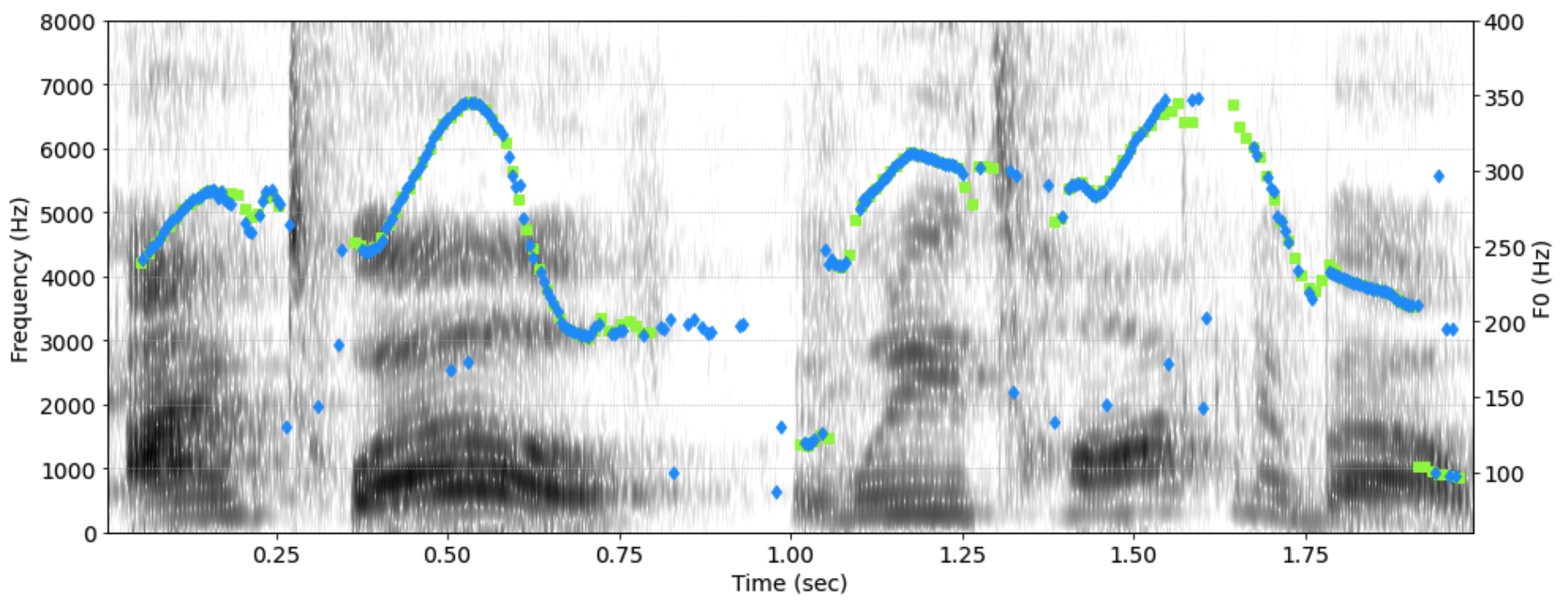
Comparing the f0 found by phon.get_f0_acd() plotted with blue diamonds, and the f0 values found by parselmouth to_Pitch(), plotted with chartreuse dots.

phonlab.get_f0_srh(y, fs, f0_range=[60, 400], isResidual=False, l=0.06, s=0.005, vthresh=0.07)

Track the fundamental frequency of voicing (f0), using a frequency domain method.

This function is an implementation of Drugman and Alwan’s (2011) “Summation of Residual Harmonics” (SRH) method of pitch tracking. The signal is downsampled to 16 kHz, and inverse filtered with LPC analysis to remove the influence of vowel formants. Then harmonics are found in the spectrum of the residual signal. Drugman and Alwan found that this technique provides an estimate of F0 that is robust when the audio signal is corrupted by noise.

The f0 range is adaptively adjusted.

Probability of voicing is given from a logistic regression formula using rms and srh trained to predict the voicing state as determined by EGG data using the function phonlab.egg_to_oq() over the 10 speakers in the ASC corpus of Mandarin speech. The prediction of the EGG voicing decision was about 84% correct.

Parameters:

• y (string or ndarray) – A one-dimensional array of audio samples

• fs (int) – Sampling rate of x

• f0_range (list of two integers, default = [60,400]) – The lowest and highest values to consider in pitch tracking. This algorithm is quite sensitive to the values given in this setting.

• isResidual (Boolean, default = False) – If the input array is a residual signal

• s (float, default = 0.005) – “Hop” interval between successive analysis windows. The default is 5 milliseconds

Returns:

df – measurements at 5 msec intervals.

Return type:

pandas DataFrame

Note

The columns in the returned dataframe are for each frame of audio:

• sec - time at the midpoint of each frame

• f0 - estimate of the fundamental frequency

• rms - rms amplitude in the band from 0 to 5 kHz

• srh - value of SRH (normalized sum of the residual harmonics)

• probv - estimated probability of voicing

• voiced - a boolean decision based on the srh value (see Drugman and Alwan)

References

20. Drugman, A. Alwan (2011) Joint robust voicing detection and pitch estimation based on residual harmonics. ‘ISCA (Florence, Italy)’ pp. 1973ff

phonlab.pitch_to_df(obj, ts=None, unit='HERTZ', interpolation='LINEAR', tcol='sec')

Return pitch values from a Praat Pitch object as a dataframe.

Parameters:

• obj (Praat Pitch obj) – The Pitch object produced by parselmouth.Sound(‘wavefile.wav’).to_pitch().

• ts (DataFrame, Iterable of floats, or None (default)) – If None (default), then the Pitch object’s ts times are used to query for pitch measurements. These are the centers of the analysis frames. The Pitch object’s values can also be queried at specific times by providing an Iterable of floats, such as a numpy array or Python list.

• unit (str 'HERTZ' (default), 'HERTZ_LOGARITHMIC', 'MEL', 'LOG_HERTZ', 'SEMITONES_1', 'SEMITONES_100', 'SEMITONES_200', 'SEMITONES_440', 'ERB'.) – The unit in which pitch values are returned. Lower case versions of the units are allowed. See Praat’s Pitch_enums.h file for defined values.

• interpolation (str 'LINEAR' (default), 'NEAREST') – The type of interpolation to use when returning values. Lower case versions of the units are allowed. See Praat’s Pitch.cpp and Vector_enums.h` files for defined values.

• tcol (str (default 'sec') or None) – The label of the time column in the output dataframe, ‘sec’ by default. If None, no time column is added to the dataframe.

Returns:

The output dataframe contains a column of pitch measurements labelled f0. The time column is labelled by the value of tcol (default ‘sec’), or omitted if tcol is None. If ts is a dataframe, the output is a concatenation of the input dataframe and the pitch measures.

Return type:

DataFrame

Examples

snd = parselmouth.Sound(mywav)
pitch = snd.to_pitch()

hzdf = phon.pitch_to_df(pitch)  # Get dataframe of pitch in Hz.

meldf = phon.pitch_to_df(pitch, unit='mel')  # or, get dataframe of pitch in mel.

##  Now you can use all of the Pandas functions with your Praat data

hzdf.to_csv('hzpitch.csv', sep='       ', header=True, index=False)
hzdf.to_pickle('melpitch.zip')

Voice Quality

phonlab.h2h1(resid, fs, f0df, f0med=None, use_ac=True)

Estimate the amplitude ratio of harmonic 2 and harmonic 1, in decibels. This function uses the method described by Drugman, Kane & Gobl (2012), and was inspired by the matlab function get_creak_h2h1() published in the Covarep Matlab repository of speech analysis software. The h2h1 measurements given by this function are correlated with those produced by phonlab.get_f0_acd() but the measurements from h2h1() should be used when testing for creaky voice.

The method here is to:

• apply a narrow (150Hz) filter centered on the f0med, to the LPC residual (see phonlab.lpcresidual())

• produce an autocorrelation of each frame

• produce a spectrum of the autocorrelation function

• based on the measured F0 for the frame, pick the spectral peaks closest to F0 and 2*F0

• and report the amplitude difference between them (the H2-H1 amplitude difference).

Drugman et al. (2012) reported that H2H1 > 0dB is a reliable indicator of creaky voice.

Parameters:

• resid (ndarray) – A one-dimensional array of lpc residual samples, as produced by phon.lpcresidual()

• fs (int) – the sampling rate of the audio in resid.

• f0df (Dataframe) – A Pandas dataframe produced by one of the get_f0 functions

• f0med (float, default = None) – Normally the median f0 is computed from the f0 values in f0df with the line: f0med = np.nanmedian(f0df.f0), but this parameter lets the user supply an estimate of the median f0 explicitly.

• use_ac (boolean, default = True) – Following Drugman et al. (2012), the function by default finds H1 and H2 in the spectrum of the autocorrelation function.

Returns:

df – The input dataframe f0df is returned with a new column h2h1

Return type:

Dataframe

References

20. Drugman, J. Kane, C. Gobl (2012) Resonator-based Creaky Voice Detection. INTERSPEECH 2012, ISCA’s 13th Annual Conference Portland, OR, USA, September 9-13, 2012

Example

example_file = importlib.resources.files('phonlab') / 'data/example_audio/sf3_cln.wav'
x,fs = phon.loadsig(example_file,chansel=[0])

x,fs = phon.prep_audio(x, fs, target_fs=16000, pre = 0, quiet=True)  # resample, scale
resid,fs = phon.lpcresidual(x,fs)
f0df = phon.get_f0_ac(x,fs)

df = h2h1(resid,fs,f0df)  # <- using information from lpcresidual(), and get_f0_ac()

# ---- Now plot the results -------
ret = phon.sgram(x,fs,cmap="Grays") # draw a spectrogram of the sound
ax2 = ret[0].twinx()
ax2.plot(df.sec,df.h2h1,'bd')
ax2.axhline(0,color="red")  # Drugman et al. use 0dB as the threshold for creaky voice

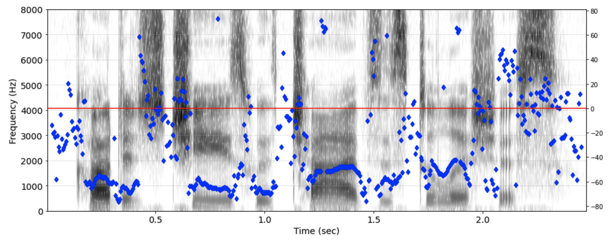
A trace of the h2h1 ratio as calculated from the LPC residual signal by phon.h2h1(). The red line at 0 dB marks a proposed threshold for classifying vocal fold vibration as creaky versus modal.

phonlab.gci_sedreams(x, fs, f0median=170, target_fs=16000, order=None, cthresh=0.0)

Identify Glottal Closure instances (GCI) using Drugman & Dutoit’s (2009) sedreams algorithm which was published as a Matlab function in the Covarep repository. The function also returns f0 and vocal jitter based on the derived GCI estimates. Two parameters are given here which were not a part of the original implementation. Based on a comment in D&D(2009), the function includes a process to choose different LPC orders for different f0medians.

low_order = int(fs/1000) + 2  # at 16kHz sampling this is 18

if order==None:
    if f0median<190: order = low_order
    elif f0median<250: order = low_order-2
    elif f0median<300: order = low_order-4
    else: order = low_order-6

If you don’t explicitly specify and LPC order one will be chosen for you. This differs from D&D in that they just used order=18 for everything. This doesn’t seem to change much in the operation of this function.

The other additional parameter is a threshold for peaks in the residual function. Changing this parameter changes the output of the function quite a lot. The algorithm looks for a peak in a temporal span of the residual in each presumed glottal cycle and reports the location of that peak as the location of the glottal closing instant, and height of the peak as the SOE (strength of excitation). With the cthresh parameter the user is given the option of disregarding intervals that have weak evidence of a glottal closure. D&D used cthresh=0, resulting in a lot of apparent jitter in regions where the actual f0 is much lower than f0median. If you add a threshold, the algorithm rejects candidate GCIs for which there is weak evidence of glottal closure. This may be a mistake for breathy voice. Further testing is needed.

Parameters:

• x (ndarray) – A one-dimensional array of audio samples

• fs (int) – sampling rate of x

• f0median (float, default = 200) – The median of the fundamental frequency of voicing in x. This value can be estimated by the user, but it is best to measure the median of values given by a pitch tracker.

• target_fs (int, default=16000) – the sampling rate of the returned residual and mbs waveforms.

• order (int, default = None) – By default the order used in LPC analysis (to calculate the LPC residual signal) is guessed based on the value of F0median. Drugmand & Dutoit (2009) used order=18.

• cthresh (float, default = 0.1) – A peak in the LPC residual must be greater than this thresholf value in in order to be considered a glottal closure instant. The residual is amplitude normalized to the range [0,1], so 0.1 is 10% of the amplitude range.

Returns:

• df (pandas DataFrame) – See the note below

• mbs (ndarray) – A waveform the same length as the input x containing the “Mean Based Signal”

• resid (ndarray) – A waveforem the same length as the input x containing the LPC residual signal.

Note

The columns in the returned DataFrame are:

• sec - the time points (in seconds) of each glottal closure instant. These are the GCI times.

• f0 - pitch of voicing, which is 1/t, where t is the glottal period - the duration between adjacent GCI times.

• jitter - the relative discrepancy between adjacent glottal period durations (call them t1 and t2). The value is calculated as j = 2 * |0.5 - t1/(t1+t2)|. This results in values on a scale from 0 (adjacent periods (t) are equal in duration), to 1 (the theoretical limit of jitter). A value of 0.5 means that t1 is twice (or 1/2) as long as t2. This corresponds to 1/2 of Praat’s “local jitter” measurement (which is scaled from 0 to 2).

• soe - strength of excitation (SOE)is the height of the LPC residual peak for each GCI

• shimmer - relative discrepancy between adjacent glottal SOE, measured in dB with the formula: shimmer = 20*log(soe[i+1]/soe[i])

References

20. Drugman, T. Dutoit (2009) Glottal Closure and Opening Instant Detection from Speech Signals, Interspeech09, Brighton, U.K.

20. Drugman, M. Thomas, J. Gudnason, P. Naylor, T. Dutoit (2012) Detection of Glottal Closure Instants from Speech Signals: a Quantitative Review, IEEE Transactions on Audio, Speech and Language Processing, vol. 20, Issue 3, pp. 994-1006.

Example

The example here shows glottal closure instances for a small 40 millisecond window in one of the exaample audio files.

example_file = importlib.resources.files('phonlab') / 'data/example_audio/im_twelve.wav'
x,fs = phon.loadsig(example_file, fs=16000,chansel=[0])
f0df = phon.get_f0_B93(x,fs)
f0med = np.nanmedian(f0df.f0)

gci_df, mbs,resid = gci_sedreams(x,fs,f0med, cthresh = 0.01)

times = np.array(range(len(x)))/fs  # construct a time axis for plotting
start = 1.8                         # choose a chunk
end = start+0.04
s = int(start*fs)
e = int(end*fs)
plt.plot(times[s:e], x[s:e]+0.75)   # plot the sound wave (centered on y = 0.75)
plt.plot(times[s:e], mbs[s:e])      # the meanbased signal
plt.plot(times[s:e], resid[s:e],'c-')  # the lpc residual
plt.vlines(np.ma.masked_outside(gci_df.sec, start,end),0.4,1.1,color='red')
plt.axhline(0.1)
plt.axhline(-0.1)

The figure here shows the derived waves used in finding GCIs. In the top trace, the sound wave is shown in blue and the glottal closure instants (GCIs) are shown with red vertical lines. In the bottom trace, the mean-based signal is shown in orange and the LPC residual is in cyan. Horizontal lines show the threshold (cthresh=0.1) for considering a peak in the residual to be a possible GCI.

phonlab.compute_cepstrogram(x, fs, dBscale=True, l=0.04, s=0.005)

Compute a cepstrogram of an audio signal. Cepstral analysis was introduced by Bogert et al. (1963). Sounds (such as voiced vowels) that have a harmonic structure, with peaks of amplitude at integral multiples of the fundamental frequency will have a strong peak in the cepstrum at the period of the fundamental. The cepstrum is computed as the spectrum of the spectrum to discover the harmonic structure of the spectrum.

Parameters:

• x (ndarray) – A one-dimensional array of audio samples

• fs (int) – Sampling rate of x

• dBscale (boolean, default = True) – Scale the cepstrum in dB

• l (float, default = 0.04) – Length of analysis windows. The default is 40 milliseconds.

• s (float, default = 0.005) – Step size, of hops between analysis windows. The default is 5 milliseconds.

Returns:

• quef (ndarray) – A one dimensional numpy array with Quefrency values (in ms)

• sec (ndarray) – A one dimensional numpy array with frame time points (in seconds)

• Sxx (ndarray) – A two dimensional numpy array with cepstral magnitudes at these timepoints and quefrencies.

References

2. 16. Bogert, M. J. R. Healy, and J. W. Tukey, (1963) The Quefrency Alanysis [sic] of Time Series for Echoes: Cepstrum, Pseudo Autocovariance, Cross-Cepstrum and Saphe Cracking, `Proceedings of the Symposium on Time Series Analysis (M. Rosenblatt, Ed) Chapter 15, 209-243. New York: Wiley.

phonlab.CPP(x, fs, target_fs=16000, smooth=2, norm=True, dBscale=True, f0_range=[60, 400], l=0.04, s=0.005)

Measure Cepstral Peak Prominence - an acoustic measure that has been shown to be highly correlated with perceived breathy vocal quality (Hillenbrand & Houde, 1996). This implementation drew inspiration and ideas from John Kane’s cpp() matlab function in the covarep repository.

Parameters:

• x (ndarray) – A one-dimensional array of audio samples

• fs (int) – Sampling rate of x

• target_fs (int, default = 16000) – Sampling rate for the analysis algorithm.

• smooth (float, default = 2) – The sigma value of a Gaussian filter that smooths the cepstrogram in both frequency and time

• norm (boolean, default = True) – Flag to request that the cepstral peak prominence be normalized for overall amplitude, using a linear fit to the cepstrum and measuring the height of the peak above the fit line.

• dBscale (boolean, default = True) – Scale the cepstrum in dB

• f0_range (an array of two numbers, default=[50,500]) – The expected range for f0.

• l (float, default = 0.04) – Length of analysis windows. The default is 40 milliseconds.

• s (float, default = 0.005) – Step size, of hops between analysis windows. The default is 5 milliseconds. If smoothing==True, the step size is reduced to 0.002 (2 millisecond).

• return_Sxx (boolean, default = False) –

  flag to request to return the cepstrogram (produced by compute_cepstrogram()) instead of returning an analysis dataframe. If smoothing is requested the smoothed cepstrogram is returned. The return values (instead of the dataframe described below) are then:

  • quef - A one dimensional numpy array with Quefrency values (in ms)

  • sec - A one dimensional numpy array with frame time points (in seconds)

  • Sxx - A two dimensional numpy array with cepstral magnitudes at these timepoints and quefrencies.

Returns:

df – measurements at 5 msec intervals.

Return type:

pandas DataFrame

Note

The columns in the returned dataframe are for each frame of audio:

• sec - time at the midpoint of each frame in seconds

• f0 - estimate of the fundamental frequency in Hz

• cpp - cepstral peak prominence in dB

Note

The default parameter values are an implementation of Hillenbrand and Houde (1996), for the measurement of breathy voice. Lower values of cepstral peak prominence are associated with breathy phonation. Following H&H, the algorithm uses smoothing both across time and quefrency to improve the identification of the cepstral peak that corresponds to the period of the voicing fundamental.

References

10. Hillenbrand, R.A. Houde (1996) Acoustic Correlates of Breathy Vocal Quality: Dysphonic Voices and Continuous Speech Journal of Speech and Hearing Science Research, 39, 311-321.

2. 16. Bogert, M. J. R. Healy, and J. W. Tukey, (1963) The Quefrency Alanysis [sic] of Time Series for Echoes: Cepstrum, Pseudo Autocovariance, Cross-Cepstrum and Saphe Cracking, Proceedings of the Symposium on Time Series Analysis (M. Rosenblatt, Ed) Chapter 15, 209-243. New York: Wiley.

Example

This example plots the cepstral peak prominence through the “I’m twelve” example recording. Note the increase in breathiness (decrease in cpp in each of the first two words “I’m” and “twelve”.

example_file = importlib.resources.files('phonlab') / 'data/example_audio/im_twelve.wav'
x,fs = phon.loadsig(example_file,chansel=[0])

cppdf   = phon.CPP(x,fs)
cpp,s,_ = phon.smoothn(cppdf.cpp,s=35,isrobust=True)  # smooth the cpp curve

ret = phon.sgram(x,fs,cmap="Blues") # draw the spectrogram from the array of samples
ax2 = ret[0].twinx()
ax2.plot(cppdf.sec, cpp, 'r-')
plt.ylabel("Cepstral Peak Prominence (dB)")

phonlab.HNR(x, fs, f0_range=[64, 400], l=0.06, s=0.005, target_time=None)

Compute the Harmonics-to-Noise Ratio using the Cepstrum-Based method given by de Krom (1993). The matlab implementation by Yen-Liang Shue (2009) which is a part of the VoiceSauce collection of software provided some valuable pointers in how to implement de Krom’s method. One difference between the Shue implementation and this one is that here we use a fixed window size (specified with the input parameter l and by default 60 ms) where Shue’s algorithm required that F0 estimates be provided as input and then HNR is calculated over windows of variable length, always long enough for 5 pitch periods according to the estimated F0 for that location in the audio.

de Krom’s (1993) method uses cepstral analysis to filter out the harmonic component of the spectrum, allowing the separate calculation of harmonic and non-harmonic energy.

Parameters:

• x (ndarray) – A one-dimensional array of audio samples

• fs (int) – Sampling rate of x

• f0_range (an array of two numbers, default=[64,400]) – The expected range for f0.

• l (float, default = 0.06) – Length of analysis windows. The default is 60 milliseconds.

• s (float, default = 0.005) – Step size, of hops between analysis windows. The default is 5 milliseconds.

• target_time (float, default = None) – If a time value (in seconds) is given, diagnostic matplotlib plots of the spectrum and cepstrum will be produced.

Returns:

df – measurements at (by default) 5 msec intervals.

Return type:

pandas DataFrame

Note

The columns in the returned dataframe are for each frame of audio:

• sec - time at the midpoint of each frame in seconds

• f0 - estimate of the fundamental frequency in Hz

• hnr_500 - The harmonics-to-noise ratio in the spectrum below 500Hz

• hnr_1500 - The harmonics-to-noise ratio in the spectrum below 1500Hz

• hnr_2500 - The harmonics-to-noise ratio in the spectrum below 2500Hz

References

7. de Krom (1993) A Cepstrum-Based Technique for Determining a Harmonics-to-Noise Ratio in Speech Signals. Jounral of Speech and Hearing Research 36,254-266.

Example

example_file = importlib.resources.files('phonlab') / 'data/example_audio/sf3_cln.wav'
x,fs = phon.loadsig(example_file,chansel=[0])

df = HNR(x,fs, target_time=2.1)  # get diagnostic plots for the spectrum at time 2.1 seconds.

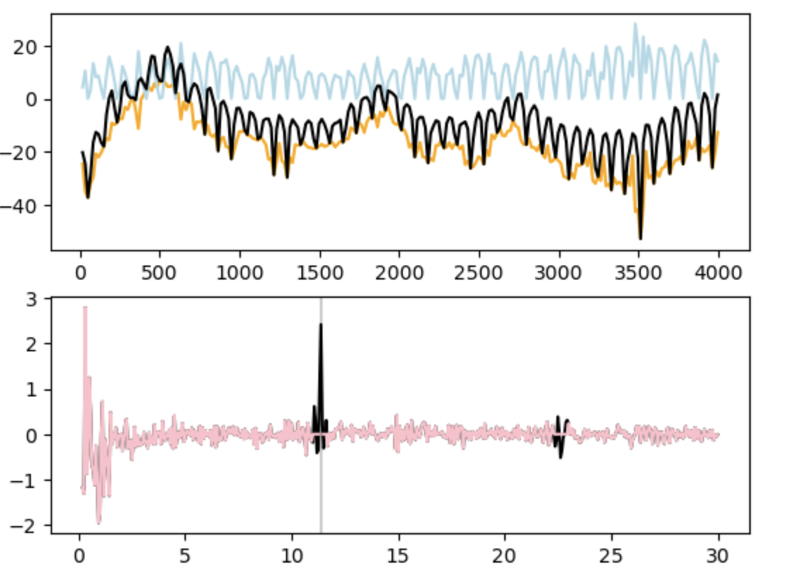
This example shows diagnostic plots of the spectrum (top panel) and cepstrum (bottom panel) of a frame of audio at time 2.1 seconds in the file ‘sf3_cln.wav’. In the top panel we see the log magnitude spectrum in black, the noise component of the spectrum in orange, and the harmonic component in light blue. In the bottom panel we see the cepstrum of the log magnitude spectrum. The “Rahmonics” in black are removed (set to zero) giving the “liftered” cepstrum (in pink). The FFT of this liftered cepstrum gives the noise spectrum (well, after some level correction).

phonlab.lpcresidual(y, fs, target_fs=16000, order=18, l=0.04, s=0.005, window='cosine')

Compute the residual signal which results from filtering the input array y using LPC inverse filtering. This signal is useful in voice quality and periodicity routines.

The LPC order is equal to (target_fs/1000) + 2, which is by default is 18.

Parameters:

• y (ndarray) – A one-dimensional array of audio samples

• fs (int) – Sampling rate of y

• target_fs (int, default = 16000) – Algorithms from the covarep library of voice analysis routines require target_fs=16000

• order (integer, default = 18) – The “order” of the LPC analysis. The number of coefficients to use in the LPC analysis. The default value is that recommended by Drugman, Kane, and Gobl (2013) for voice quality analysis (fs/1000 + 2), with the caveat that a smaller number may be more appropriate for voices with higher fundamental frequency.

• l (float, default = 0.04) – The duration of the LPC analysis window, 40 milliseconds

• s (float, default = 0.005) – The interval between successive frames in the LPC analysis, 5 milliseconds

• window (str, tuple, numeric, callable, list-like (default 'hann')) – Window function applied to each frame. This parameter is passed as the window parameter to scipy.signal’s get_window function.

Returns:

• lpc_residual (ndarray) – A one-dimensional array – the residual derived by inverse filtering the input audio signal. It has the same number of samples as the input y array.

• fs (int) – The sampling rate of lpc_residual. It will be the same as target_fs, which by default is 16000 Hz.

phonlab.overlap_add(frames, hop_length, window_vec)

Perform Overlap-Add reconstruction from 2D frames to a 1D signal.

Parameters:

• frames (ndarray) – A 2D array of shape (n_frames, frame_length)

• hop_length (int) – Number of samples to shift for each frame

• window_vec (1D array (frame_length)) – use scipy.signal.windows to get this vector with a statement like win = windows.get_window(‘cosine’, Nx=frames.shape[1], fftbins=False)

Returns:

y – The reconstructed 1D signal.

Return type:

ndarray

Consonant Features

phonlab.fricative(x, fs, t)

Measure fricative acoustic values, from a 20 ms window, centered on time t.

In addition to reporting the spectral moments (COG, SD, skew, and kurtosis) of the multitaper spectrum (from nitime.algorithms.multi_taper_psd()), fricative() finds the “main peak” in the fricative spectrum. For fricatives with a resonant cavity, this is the lowest resonance of the cavity. For those with no resonance the main peak frequency may be more a property of the source function.

The main peak heuristic is to start by looking the in the spectrum above 300 Hz, for the lowest frequency peak that is at least 50% of the amplitude range, separated from the nearest peak by at least 500Hz, and prominent by 8bB above the next nearest peak (see the scipy.signal.find_peaks() documentation). If no peak is found, relax the prominence constraint, then the amplitude constraint, and then both.

Parameters:

• x (ndarray) – a one-dimensional array of audio samples

• fs (int) – the sampling frequency of x (ideally should be at least 16000)

• t (float) – the time (in seconds) at which to take measurements (this is usually in a fricative, but doesn’t have to be).

Returns:

A FricMeas namedtuple of fricative measures is returned, with the following fields:

Fmfloat

Frequency (in Hz) of the first main spectral peak. A measure correlated with the length of the front tube.

Amfloat

Amplitude (in dB) at Fm

AmpDfloat

The difference in amplitude (dB) between the higher of Am or Asec and the minimum amplitude between 500Hz and Fm. A measure of sibilance.

Fsecfloat

Frequency of the second major peak in the spectrum. If the front tube is long there can be a second resonance. If there is no second major peak, this field’s value is None

Asec: float

Amplitude (in dB) at Fsec. If there is no second major peak, this field’s value is None

modestring

a report on the peak finding parameters used

COGfloat

center of gravity, the first moment of the spectrum.

SDfloat

standard deviation, the second moment of the spectrum.

Skewfloat

scaled third moment, skew

Kurtosisfloat

scaled fourth moment, kurtosis

specndarray

the multi-taper power spectrum at the midpoint (e.g. for use in plotting spectra)

freqndarray

the frequency scale of the spectrum (e.g. for use in plotting spectra)

Return type:

namedtuple

Note

The major peaks analysis implemented here draws on ideas from Shadle (2023) and Shadle et al. (2023). Moments analysis was introduced for analysis of stop release burst spectra by Forrest et al. (1988).

References

11. Forrest, G. Weismer, P. Milenkovic, and R.N. Dougall (1988) Statistical analysis of word-initial voiceless obstruents: Preliminary data. J. Acoust. Soc. Am. 84(1), 115–123.

3. Shadle (2023) Alternatives to moments for characterizing fricatives: Reconsidering Forrest et al. (1988). J. Acoust. Soc. Am. 153 (2): 1412–1426. https://doi.org/10.1121/10.0017231

3. Shadle, W-R. Chen, L.L. Koenig, J.L. Preston (2023) Refining and extending measures for fricative spectra, with special attention to the high-frequency range. J. Acoust. Soc. Am. 154 (3): 1932–1944. https://doi-org.libproxy.berkeley.edu/10.1121/10.0021075

Example

This example returns fricative measurements from time 2.25 seconds in the audio samples returned by loadsig(). The major peak and COG frequencies are indicated in a plot of the spectrum.

x, fs = phon.loadsig("sf3_cln.wav")
y, fs = phon.prep_audio(x, fs, target_fs=16000)
fricm = phon.fricative(y, fs, 2.25)

print(f"first major peak at {fricm.Fm:.1f}, Center of Gravity is {fricm.COG:.1f}")
plt.plot(fricm.freq, fricm.spec)
plt.axvline(fricm.Fm, color="red")
plt.axvline(fricm.COG, color="green")

The figure here shows major peaks and COG in several different fricatives.

Marking major peaks (red lines) and COG (green line) in fricative spectra.

phonlab.burst(x, fs, start, end)

Find a stop burst in a short interval of audio

This function takes an array of waveform samples and returns the location in time of the most prominent stop release burst in a segment of audio indicated by the start and end parameters. Generally, start and end are taken from a TextGrid and define a short (50ms to 150ms) segment that has been labeled as containing a consonant of interest (a stop, fricative or nasal for example). In addition to the time of the strongest burst in the time-span, a burst strength score is also returned.

The algorithm looks at sudden peaks in the acoustic waveform that correspond to a large change in the mel frequency spectrum (a sudden increase in spectral energy) and scores each candidate with a linear discriminant formula that was trained on TIMIT stop release bursts. The time and score of the winning candidate is returned.

Parameters:

• x (ndarray) – a one-dimensional array of waveform samples

• fs (number) – the sampling frequency of the audio in x. The algorithm was trained on speech sampled at 16000 Hz, and will work best if you resample to 16000 with phon.prep_audio() before calling this function. See the example.

• start (float) – the time in seconds at the start of the waveform chunk in x

• end (float) – the time in seconds at the end of the waveform chunk in x

Returns:

• b_time (float) – the time in seconds of the most prominent burst in x between start and end

• b_score (float) – a measure of the prominence of the burst

Example

In this example we open a sound file with phon.loasig(), prepare it for the burst detector with phon.prep_audio() and then search for the best candidate for a stop release burst in the interval from time 1.5 seconds to time 2.0 seconds. The return value b_time is the location of the burst in seconds, and b_score is a measure of the burst prominence. The sgram() plot in this example illustrates the use of start and end to produce a spectrogram of a specified portion of signal.

x,fs = phon.loadsig("sf3_cln.wav", chansel=[0])
x,fs = phon.prep_audio(x,fs, target_fs=16000, pre=0.94)

t1 = 1.5
t2 = 2

b_time, b_score = phon.burst(x,fs,t1,t2,fs)  # find a stop burst in the span from t1 to t2

ax1,f,t,Sxx = phon.sgram(x,fs_in=fs,start=t1, end=t2)
ax1.axvline(b_time,color="red")

Marking the burst found by phon.burst()

phonlab.nasality(x, fs, order=18, analysis_band=(80, 2500), acoustic_spectrum='CEP', smoothing_factor=None, preemphasis=0.96, length=0.04, step=0.005, lift=0.0025, target_fs=12000, slice_time=-1, verbose=False)

This function implements an idea in Johnson (Acoustic and Auditory Phonetics) that vowel nasality may be indicated by the spectral cosine difference (SCD) between the LPC spectrum (which assumes non-nasality) and a spectrum with fewer assumptions (a narrow-band FFT or a cepstrally smoothed spectrum).

The idea is that because nasality introduces antiformants and/or additional resonant peaks in the spectrum of a vowel, nasalized vowels should have a greater difference between the LPC spectrum and an acoustic spectrum than the SCD we will find in non-nasalized vowels.

In this function phon.RLPC_formants() is used to to produce LPC spectra, phon.compute_sgram() is used to compute narrow-band spectra, and phon.cepstral_smooth() is used to produce cepstrally smoothed spectra. The function then reports the spectral cosine difference (SCD) (in the specified analysis band) between the LPC spectrum and either the cepstrally smoothed acoustic spectrum or the raw (FFT) narrow-band acoustic spectrum.

In addition the function returns two commonly used measures of vowel nasality: the bandwidth of F1 from the RLPC function, and the difference between the amplitude of the harmonic closest to F1 and the lowest harmonic.

Parameters:

• x (ndarray) – a 1D array of audio samples

• fs (int) – the sampling rate of samples in x. This will be resampled to ‘target_fs’ for analysis, so choose the order paramter with this in mind.

• order (integer (default = 18)) – Number of LPC coefficients, passed to RLPC_formant(). The default value is rather large, allowing the LPC function to capture more peaks and valleys than may be typical in vowel formant tracking analyses. You can set this parameter to -1 and then the function choose_order() will be used to determine the value for this parameter.

• analysis_band (list, default = (80,2500)) – Compute the spectral difference over this frequency band (in Hz)

• acoustic_spectrum (string, default = "CEP") – Which acoustic spectrum to compare with the LPC spectrum. Allowable values are “FFT” for the narrow-band FFT, or “CEP” for the cepstrally smoothed spectrum. The default approach, using the cepstrally smoothed spectrum seems to be less affected by voice pitch effects.

• smoothing_factor (float, default = None) – If the value of this parameter is less than zero, then no smoothing will be done. Otherwise this is the s parameter to be passed to phon.smoothn() to robustly smooth the data. Note that passing None (the default action) will have smoothn() automatically determine a smoothing factor for each trajectory and in verbose mode will report the value of the choosen smoothing factor. See smoothn for more information.

• preemphasis (float, default = 0.96) – value of a preemphasis factor (0-1).

• length (float, default = 0.04) – duration (in seconds) of analysis frames, the default of 0.04 gives a narrowband spectrum with resolution appropriate for resolving harmonics.

• step (float, default = 0.005) – the interval (in seconds) between successive formant measurements.

• lift (float, default = 0.0025) – The cepstral smoothing filtering coefficient (in seconds). Compenents that have a period longer than the lift value will be removed from the signal. This is used in cepstral smoothing to remove source spectral characteristics and keep vocal tract filter effects. The default value of 2.5 ms means that cepstral components lower than 400 Hz will be removed. Smaller values of this parameter lead to more cepstral smoothing, and larger values lead to less spectral cepstral smoothing.

• target_fs (int, default = 12000) – Sampling frequency at which the analysis will be done. The top frequency in the analysis is thus the Nyquist frequency (1/2 of the target_fs).

• slice_time (float, default = -1) – If a time value greater than 0 is given, then a diagnostic plot will be produced for the spectral slice at the slice_time.

• verbose (boolean, default = False) – If true, print diagnostic messages.

Return type:

df - a pandas dataframe with columns as described in the note below.

Note

The columns in the output dataframe are:

• sec - midpoint time of the frame

• F1-4 - the lowest four vowel ‘formants’ - vocal tract resonances.

• BW1-4 - bandwidths of the vowel formants

• gain - the LPC gain (variance of the residual) for each frame.

• BW1_nas - the smoothed BW1, bandwidth of F1. Larger values indicate more nasality.

• a1h1 - the difference in amplitude of the harmonic closest to F1 and the lowest harmonic. Smaller values indicate more nasality (lower amplitude F1).

• SCD - the spectral cosine distance between the LPC spectrum and the acoustic spectrum in the analysis band. Larger values indicate more nasality.

Example

This example returns nasality measurements in a dataframe, and plots example spectra at a particular slice time. The Spectral Cosine Distance and a1h1 measures are plotted on the spectrogram.

audio_dir = importlib.resources.files('phonlab') / 'data/example_audio'
example_file = audio_dir / 'FR_bon_beau.wav'
x,fs = phon.loadsig(example_file,chansel=[0])

st = 0.41

nasdf = phon.nasality(x,fs, slice_time=st, verbose=True)

# --------  plot -----------
ax = phon.sgram(x,fs,tf=5000)[0]
ax.plot(nasdf.sec,nasdf.F1,'w.')
ax.text(0.2,4500, "[ bõ ]",fontsize=18)
ax.text(0.8,4500, "[ bo ]",fontsize=18)
ax.text(1.4,4500, "[ bõ ]",fontsize=18)
ax.text(2,4500, "[ bo ]",fontsize=18)
if st >0:
    ax.axvline(st,color='red')

ax2 = ax.twinx()
ax2.plot(nasdf.sec,nasdf.SCD,'md')
ax2.set_ylim(0,16)
ax3 = ax.twinx()
ax3.plot(nasdf.sec,nasdf.a1h1,color='dodgerblue',marker='o',linewidth=0)
ax3.set_ylim(0,16)

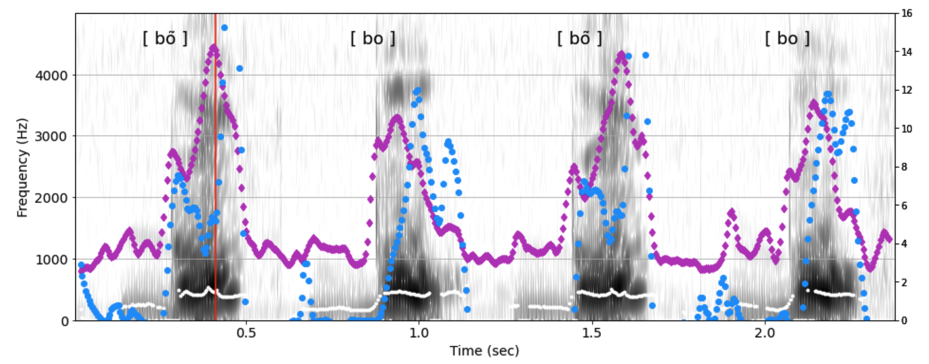
Overlaid on a spectrogram are plotted nasality measures SCD (magenta diamonds) and a1h1 (blue dots) for two repetitions of the French minimal pair <bon> and <beau>. Frequency of F1 is plotted with small white dots.

Rhythm

phonlab.get_rhythm_spectrum(x, fs)

Return a rhythm spectrum - ala Tilsen & Johnson, 2008

This approach to measuring rythmicity was described by Tilsen and Johnson (2008). The code here and in rhythmogram is a translation and extension of Tilsen’s Matlab code. This function takes a chunk of waveform (best if it is 4 seconds long) and computes a spectrum of the bandpass filtered amplitude envelope. It finds periodicity in the amplitude envelope and returns a spectrum in the range from f to 7 Hz, tracking components in the amplitude envelope that repeat at low frequency. The lowest frequency represented f is determined from the duration of the waveform in x, which should be at least 4 seconds for accurate detection of slow rhythmic components.s

Parameters:

• x (ndarray) – A one dimensional array of audio samples -

• fs (int) – The sampling frequency of x

Returns:

• freq (ndarray) – The frequency axis of the rhythm spectrum

• psd (ndarray) – The amplitude values of the rhythm spectrum

References

19. Tilsen & K. Johnson (2008) Low-frequency Fourier analysis of speech rhythm. Journal of the Acoustical Society of America, 124 (2), EL34-EL39.

Example

x,fs = phon.loadsig("s09003.wav")
slice = x[fs*3:fs*7]

f,Sx = phon.get_rhythm_spectrum(slice,fs)
plt.plot(f,Sx)

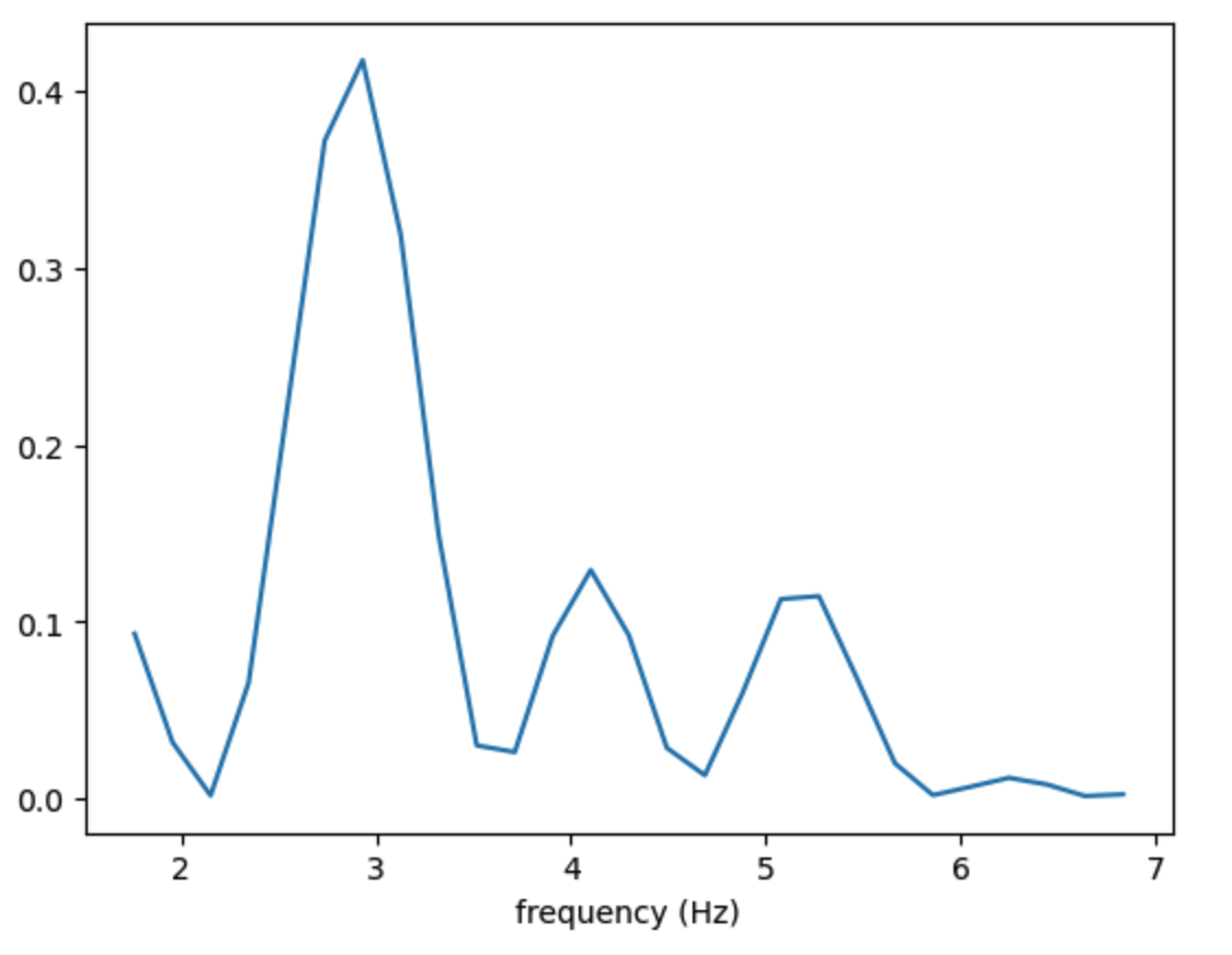
The spectrum of the amplitude envelope of a 4 second chunk of audio. This section of speech in Spanish has an oscillation of about 3 Hz; regular repetition of amplitude peaks at intervals of about 330 msec.

phonlab.rhythmogram(x, fs)

Return a rhythm spectrogram - ala Tilsen & Johnson, 2008

The approach to measuring rythmicity that is implemented by this function was described by Tilsen and Johnson (2008). The code here and in get_rhythm_spectrum is a translation and extension of Tilsen’s Matlab code. This function takes a buffer of audio and computes spectra of the amplitude envelope of the bandpass [100 - 1500Hz] filtered signal. Spectra are computed twice a second (i.e. the step size is 0.5 seconds) over windows that are 4 seconds long. It finds periodicity in the amplitude envelope and returns a spectrogram with a frequency range from 1 to 7 Hz, tracking components that repeat at intervals of once per second down to a repetition rate of 140 ms.

Parameters:

• x (ndarray) – A 1-D array of audio samples

• fs (int) – the sampling frequency of the audio in x (in Hz)

Returns:

• t (ndarray, one-dimensional) – the time axis of the rhythmogram, in seconds

• f (ndarray, one-dimensional) – the frequency axis of the rhythmogram, in Hz

• Sxx (ndarray, two-dimensional) – the amplidude values of the rhythmogram, axis 1 is time, axis 0 is frequency

References

19. Tilsen & K. Johnson (2008) Low-frequency Fourier analysis of speech rhythm. Journal of the Acoustical Society of America, 124 (2), EL34-EL39.

Example

x,fs = phon.loadsig("s1202a.wav", chansel=[0])
ts,f,Sxx = phon.rhythmogram(x,fs)  # calculate rhythm spectra over time

m = np.mean(Sxx,axis=0)  # the mean spectrum of the file
sd = np.std(Sxx,axis=0)  # the standard deviation of the spectrum
Sxx_thresh = Sxx - (m + 0.5*sd)   # subtract a threshold to find "rhythmic" sections

start = 136  # seconds, show the thresholded spectrogram for a 30 second interval
end = 166
s = np.int32((start-2) *2)  # start frame, two frames per second
e = np.int32((end-2) *2) # end frame
extent = (start,end,min(f),max(f))  # get the time and frequency values for figure.

plt.imshow(Sxx_thresh.T[:,s:e], aspect='auto', extent = extent,
      origin='lower',cmap="coolwarm",interpolation="spline36")
plt.set(xlabel="Time (sec)", ylabel="Frequency (Hz)")

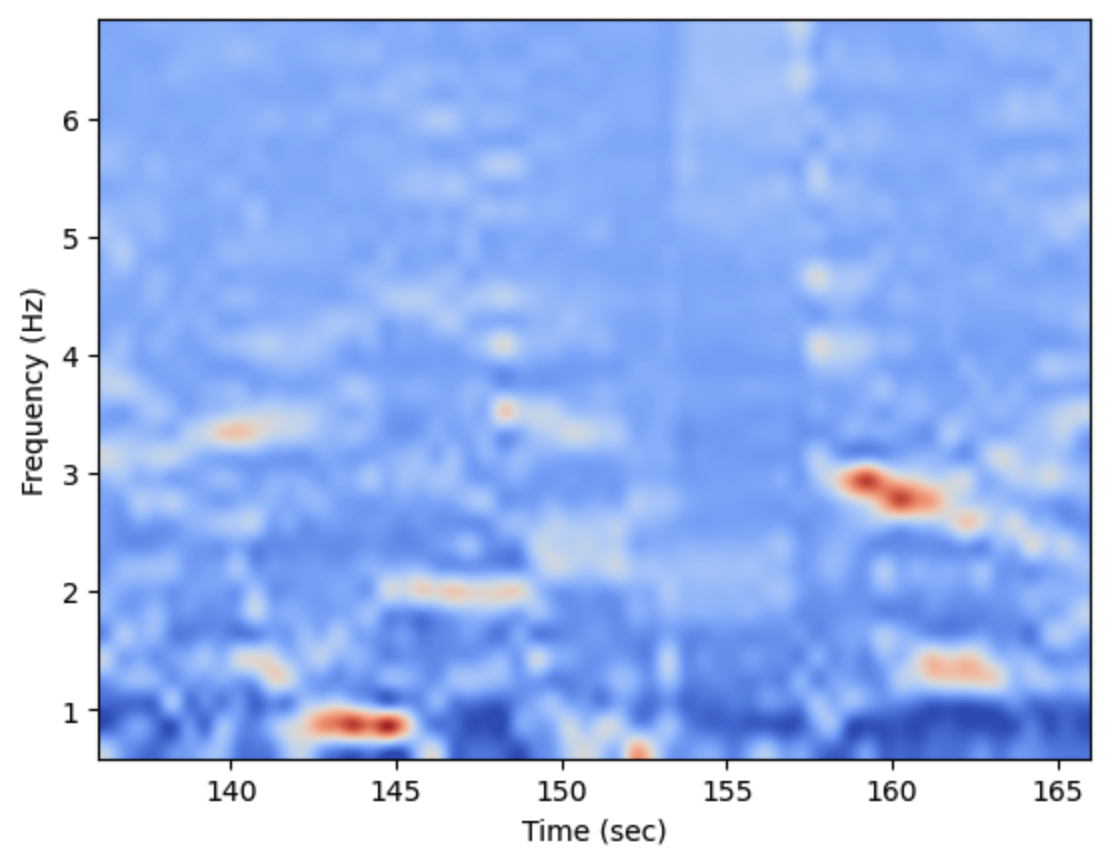
A time/frequency plot of low frequency energy in a 30 second long chunk of speech