Auditory Phonetics

Signal Manipulation

phonlab.add_noise(x, fs, noise_type='white', snr=0, target_amp=-2)

Add noise to audio

This function is partially adapted from matlab code written by Kamil Wojcicki, UTD, July 2011. It does the following:

• pads the audio signal with 1/2 second of silence at the beginning and end

• takes an audio file and mixes it with a noise (or a passed audio file) at a specified signal to noise ratio.

• scales the peak intensity of the resulting mixed audio to prevent clipping

• writes the resulting mixed audio as .wav files to an output directory

Parameters:

• x (array) – A one-dimensional array of audio samples

• fs (int) – the sampling frequency of the audio in x

• noise_type (string, default = "white") – The type of noise - one of “pink”, “white”, “brown”, ‘babble’, ‘party’, or ‘restaurant’.

• snr (float, default = 0) – the signal to noise ratio in dB. 0 means that the signal peak RMS amplitude will be the same as the noise amplitude. Less than zero (e.g. -5) means that the signal amplitude will be lower than the noise, and greater than zero means that the signal amplitude will be greater than the noise amplitude.

• target_amp (number, default = -2) – Scale the resulting signal (the result of adding the noise to the signal) so that the peak amplitude is target_amp relative to the maximum possible value. Use a negative number to avoid clipping. -2 means scale the resulting signal so that it is -2 dB below the maximum for digital audio files.

Returns:

• y (ndarray) – The result of adding noise to the signal

• fs (int) – The sampling rate of the signal in y

Raises:

ValueError – if the noise_type is not a valid type

Example

This example adds white noise at a signal-to-noise ratio (SNR) of 3 dB

x,fs = phon.loadsig("sf3_cln.wav",chansel=[0])
y,fs = phon.add_noise(x,fs,"white",snr=3)
phon.sgram(x,fs)

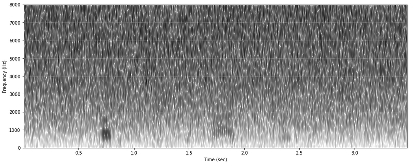
The result of adding white noise.

phonlab.sigcor_noise(x, fs, flip_rate=0.5, start=0, end=-1)

Add signal correlated noise to an audio file.

The function takes a filename and returns a numpy array that contains the signal with added signal correlated noise. This by done by flipping the polarity of samples randomly. Note that flip_rate of 0 means no change, and 1 means flip the polarity of all of the samples, 0.5 means randomly flip the polarity of 1/2 of the samples (imagine flipping a coin for each sample, heads leave it as it was, tails multiply it by -1). So, the maximum “noise” is with flip_rate = 0.5.

Parameters:

• x (ndarray) – An one-dimensional array of audio samples.

• fs (int) – the sampling frequency of the audio samples in x

• flip_rate (float, 0 <= flip_rate <= 1.0, default = 0.5) – determines the proportion of samples to flip (0.5 gives maximum noise)

• start (float, default = 0) – the time (in seconds) at which to start adding noise (default is 0)

• end (float, default = -1) – the time (in seconds) at which to stop adding noise (default is -1, apply to the end of the audio).

Returns:

• y (ndarray) – A one-dimensional array derived from x

• fs (float) – the sampling rate of y

Example

Open a file and add signal correlated noise to the section between 1.2 and 1.5 seconds.

x,fs = phon.loadsig("sf3_cln.wav",chansel=[0])
y,fs = phon.sigcor_noise(x,fs,flip_rate=0.4,start=1.2,end=1.5)

phonlab.vocode(x, fs, bands, target_fs=None)

Noise vocoding - replace sound with bandpassed noise, using a bank of filters defined by bands.

This module is based on the excellent vocoder notebook published by Alexandre Chabot-Leclerc ([@AlexChabotL](http://twitter.com/alexchabotl)). https://github.com/achabotl/vocoder.git

Keith Johnson added the “Shannon” vocoding scheme and altered some of the functions to be a little more general, and also converted the filtering to use sos coefficients, which improved the numerical stability of the code.

Parameters:

• x (ndarray) – A one-dimensional array of audio samples

• fs (int) – the sampling frequency of the audio samples in x.

• bands (list) – A list of n bandpass filter lower/upper cut off freqs (n,2), as returned by third_octive_bands() or shannon_bands()

• target_fs (int, default None) – the desired frequency of the resulting vocoded signal. None keeps the rate at the value passed in fs.

Returns:

• y (ndarray) – an array of samples, the same length as sig

• fs (int) – the sampling frequency of y

Example

example_file = importlib.resources.files('phonlab') / 'data/example_audio/sf3_cln.wav'

bands_third = phon.third_octave_bands(high=8000)  # define filter bank
bands_shan = phon.shannon_bands(high=8000,nc=10)  # define filter bank

x,fs = phon.loadsig(example_file,chansel=[0])
y,fs = phon.vocode(x, fs, bands_shan)  # use one of the filter banks

phon.sgram(y,fs)

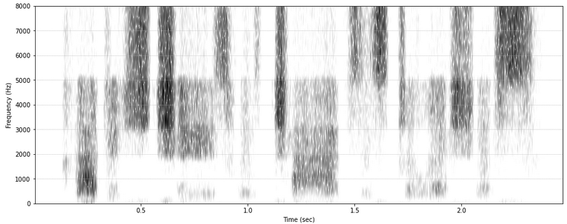
A spectrogram of Shannon vocoded speech

phonlab.sine_synth(formant_data, fs=16000)

Produces ‘sinewave speech’ - an audio signal made up of time-varying sinusoidal waves at the frequencies of the vowel formants.

Note

The input dataframe is usually produced by phonlab.track_formants() and in any case should have these columns:

• sec : Time (seconds) of the frames.

• rms : The RMS amplitude of each frame.

• F1,F2,F3,F4: Frequencies (Hz) of the lowest four vowel formants, in the frames.

The overall amplitude contour of the sine wave speech waveform is determined by the RMS contour in the input file. The frequencies of four sine wave components are given by the formant estimates in the input file.

The amplitude of the sine wave speech waveform is scaled to use the full amplitude range available with 16 bit integer samples. Also, short 20ms on-ramp and off-ramp amplitude contours are applied to the beginning and end of the audio.

This is a python translation of code that Keith Johnson got from Howard Nusbaum, via Alexander Francis, in 1998.

Parameters:

• formant_data (dataframe) – a pandas dataframe with speech analysis data as produced by phonlab.track_formants()

• fs (number, default=16000) – the sampling frequency of the resulting sound wave.

Returns:

• wav (ndarray) – a one-dimensional numpy array containing audio samples

• fs (number) – the sampling frequency of the audio samples in wav

References

18. 5. Remez, P.E. Rubin, D.B. Pisoni & T.D. Carrell (1981) Speech perception without traditional speech cues. Science 212 (4497), 947–950. doi:10.1126/science.7233191

Example

x,fs = phon.loadsig("sf3_cln.wav",chansel=[0])
fmtsdf = phon.track_formants(x,fs)    # track the formants
x,fs = phon.sine_synth(fmtsdf,fs=fs)     # produce the sinewave synthesis
librosa.output.write_wav('sf3_cln_sinewave.wav', x, fs)  # save wav file

phonlab.shannon_bands(nc=24, low=70, high=5000)

Split a frequency range (low, high) into nc (number of channels) frequency bands on log freq scale

Parameters:

• nc (int, default = 24) – the number of frequency bands in the vocoded output

• low (int, default = 70) – low frequency of the range to be covered by the channels (Hz)

• high (int) – high freq of range covered by the channels (at most fs/2 - 1)

Returns:

bands – a list of band limits for a bank of bandpass filters

Return type:

list

phonlab.third_octave_bands(low=100, high=5000)

Compute cutoff frequencies for 1/3 octave bands, the centers are spaced one octave apart

Parameters:

• low (int, default = 100) – low frequency of the range to be covered by the channels (Hz)

• high (int, default = 5000) – high freq of range covered by the channels (at most fs/2 - 1)

Returns:

bands – a list of band limits (low,high) for a bank of bandpass filters

Return type:

list

phonlab.apply_filterbank(x, bands, fs=22050, order=8)

Apply a bank of bandpass filters

Filter using repeated calls to scipy.signal.sosfiltfilt(), once for each of a bank of 8th order Butterworth bandpass filters. The output array has one copy of x for each of the bands listed in the input “bands” parameter.

Parameters:

• x (ndarray) – audio samples in a 1-D numpy array

• bands (list) – A list of c filter lower/upper cut off freq pairs (c,2)

• fs (int, default = 22050) – the sampling frequency of the sound to be filtered

• order (int, default=8) – the order of the bandpass filters (passed to scipy.signal.butter)

Returns:

y – a 2-D array of x filtered by each band, y[0] is the input filtered by bands[0]

Return type:

ndarray, shape(c,n)

Auditory Representations

phonlab.compute_mel_sgram(x, fs, step_sec=0.01)

Compute a Mel frequenc spectrogram of the signal in x. This function is adapted from the code example given in the documentation for the tensorflow function mfccs_from_log_mel_spectrograms().

Parameters:

• x (ndarray) – A one-dimensional array of audio samples

• fs (int) – The sampling rate of the audio samples in x. The tensorflow example assumed that fs=16000

• step_sec (float, default = 0.01) – The step size between successive spectral slices. The tensorflow example used t=0.016, 16 milliseconds.

Returns:

• sec (ndarray) – a one dimensional array of time values, the time axis of the spectrogram

• mel_f (ndarray) – a one dimensional array of mel frequency values - the frequency axis of the spectrogram

• mel_sgram (ndarray) – A two-dimensional (time,frequency) array of amplitufe values. The intervals between time slices is dependent on the s input parameter, by default 10 ms, and the frequencies are evenly spaced on the mel scale from 80 to 7600 Hz in 80 steps.

Example

This example uses the function to compute a log mel-frequency spectrogram, and then passes that to the tensor flow function to compute mel-frequency cepstral coefficients from it.

# Compute MFCCs from log_mel_spectrograms and take the first 13.
mel_f, sec, mel_sgram = phon.compute_mel_sgram(x,fs)
mfccs = tf.signal.mfccs_from_log_mel_spectrograms(mel_sgram)[..., :13]

The mel_sgram of the example audio file sf3_cln.wav - “cottage cheese with chives is delicious”

phonlab.mfcc_to_df(obj, num, ts=None, tcol='sec', include_energy=True)

Return mfcc values from a Praat MFCC object as a dataframe.

Parameters:

• obj (Formant obj) – An MFCC object produced by parselmouth.Sound(‘wavefile.wav’).to_mfcc().

• num (int) – The number of MFCC coefficients which will be calculated and returned in the columns labelled c1 … cN, where N is num. See the include_energy param for c0.

• ts (DataFrame, Iterable of floats, or None (default)) – If None (default), then the Formant object’s ts times are used to query for formant measurements. These are the centers of the analysis frames. The Formant object’s values can also be queried at specific times by providing an Iterable of floats, such as a numpy array or Python list.

• tcol (str (default 'sec') or None) – The label of the time column in the output dataframe, ‘sec’ by default. If None, no time column is added to the dataframe.

• include_energy (bool (default True)) – If True, include the zeroth cepstral coefficient in the column labelled`c0`. For an MFCC object this value relates to energy.

Returns:

The output dataframe contains columns of times and MFCC coefficients. The coefficient columns are labelled c1 … cN, where N is an integer. If include_energy is True, then the zeroth cepstral coefficient is also included in the c0 column. The time column is labelled by the value of tcol (default ‘sec’), or omitted if tcol is None. If ts is a dataframe, the output is a concatenation of the input dataframe and the MFCC values.

Return type:

DataFrame

Examples

ncoeff = 12
snd = parselmouth.Sound(mywav)
mfcc = snd.to_mfcc(number_of_coefficients=ncoeff)

mdf = phon.mfcc_to_df(mfcc, num=ncoeff, include_energy=True)

# Now you can use all of the Pandas functions with your Praat data

mdf.to_csv('mfcc.csv', sep='   ', header=True, index=False)
mdf.to_pickle('mfcc.zip')

class phonlab.Audspec(fs=16000, step_size=0.03)

Create an an Audspec object; analysis parameters and routines for creating auditory spectrograms.

Parameters:

• fs (int, default=16000) – The desired sampling rate of audio analysis, determines the frequency range of the auditory spectrogram. Note that if the value given here exceeds the sampling rate of the file passed, there can be ‘empty’ space at the top of the auditory spectrogram.

• step_size (float, default=0.03) – The interval (in seconds) between successive analysis frames.

Returns:

object – The object returned by the constructor function is ready for calls to functions like object.make_zgram(), object.make_sharpgram(), etc. to compute auditory representations of sound.

Return type:

Audspec

Examples

The examples here show the use of the Audspec class to create auditory representations of sounds, roughly based on the properties of the human cochlea and aspects of auditory processing in the brainstem. The most basic representation is the auditory spectrogram (internally called the zgram and sometimes referred to as the audiogram), which is simply a critical band filtered spectrogram.

x,fs = phon.loadsig("sf3_cln.wav",chansel=[0])
aud = phon.Audspec()
aud.make_zgram(x,fs)

# ---- the rest is to make a nice plot ----

fig,ax = plt.subplots(2,figsize=(6,5))

Hz_extent = (min(aud.time_axis), max(aud.time_axis),
      min(aud.fft_freqs), max(aud.fft_freqs))  # time and frequency values for sgram.
ax[0].imshow(20*np.log10(aud.sgram.T),origin='lower', aspect='auto', interpolotion="spline36",
         extent=Hz_extent, cmap = plt.cm.Greys)
ax[0].set(xlabel="Time (sec)", ylabel="Frequency (Hz)")
ax[1].imshow(aud.zgram.T,origin='lower', aspect='auto', interpolotion="spline36",
         extent=aud.extent, cmap = plt.cm.Purples)
ax[1].set(xlabel="Time (sec)", ylabel="Frequency (Bark)")
fig.tight_layout()

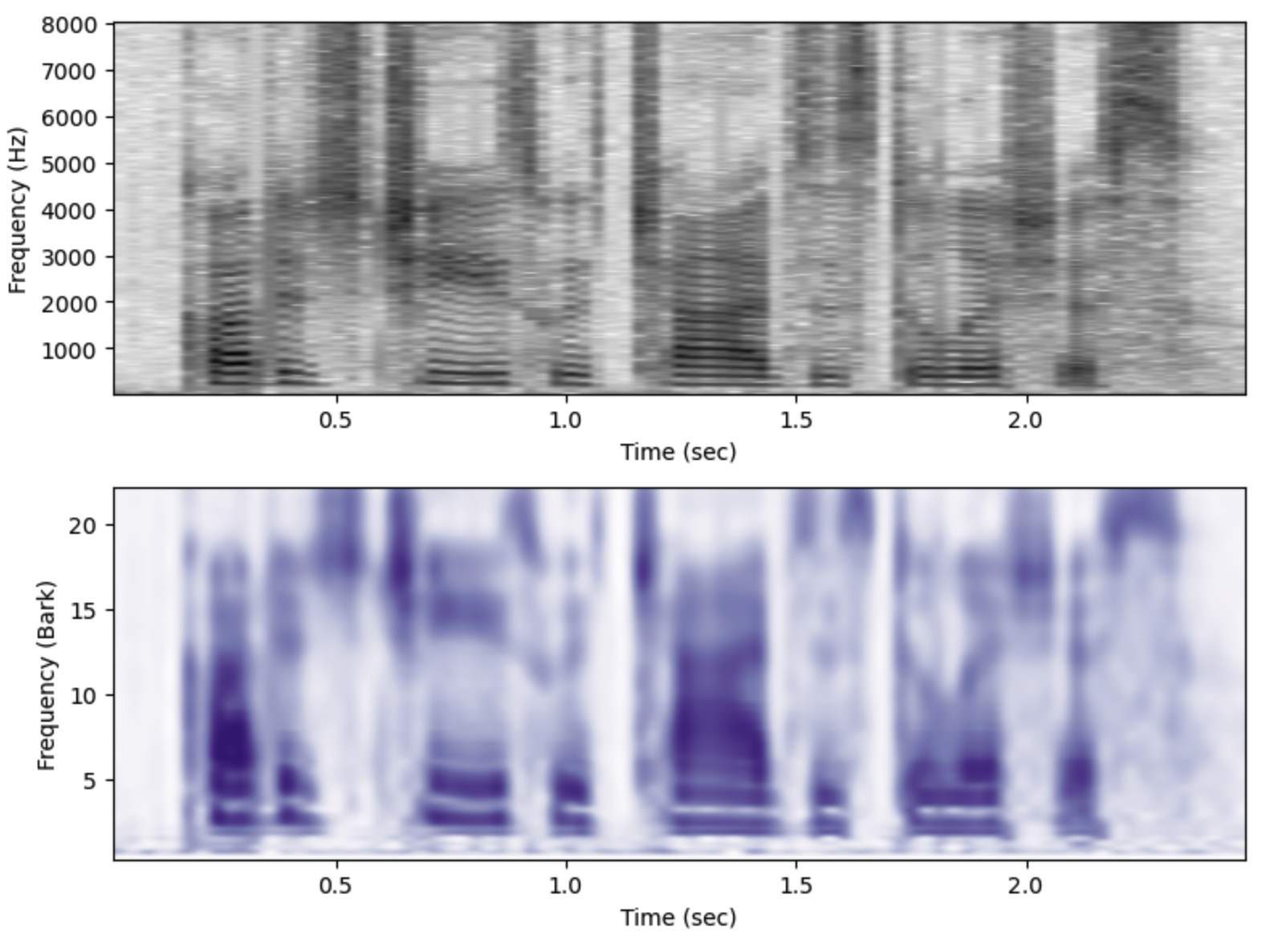
(top) Acoustic narrow band spectrogram, and (bottom) Auditory spectrogram of the same utterance.

One type of secondary auditory processing sharpens the frequencies of the audiogram, simulating frequency selectivity through lateral inhibition.

aud.make_sharpgram()
fig,ax = plt.subplots(1,figsize=(8,3))

ax.imshow(aud.sharpgram.T,origin='lower', aspect='auto',
         extent=aud.extent, interpolation="spline36", cmap = plt.cm.Reds)
ax.set(xlabel="Time (sec)", ylabel="Frequency (Bark)")

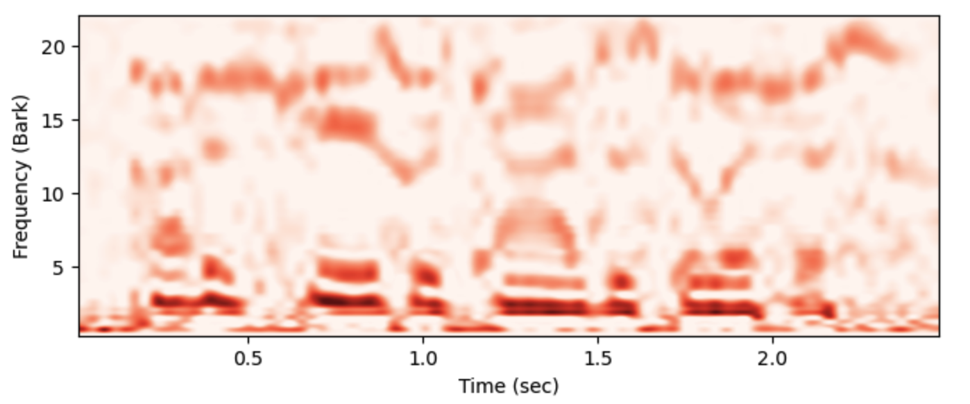
(top) The “sharpgram” auditory representation.

Another auditory representation emphasizes temporal changes in the audiogram. In the Audspec class this is referred to as a tgram.

aud.make_tgram()
fig,ax = plt.subplots(1,figsize=(8,3))

ax.imshow(aud.tgram.T,origin='lower', aspect='auto',
         extent=aud.extent, interpolation="spline36", cmap = plt.cm.afmhot)
ax.set(xlabel="Time (sec)", ylabel="Frequency (Bark)")

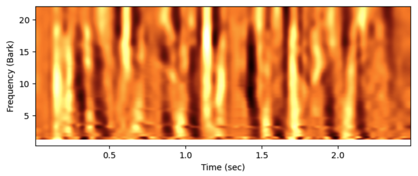
(top) The “tgram” auditory representation, showing the gradient of change in critical bands.

Methods and Attributes in an Audspec object

make_zgram(x, fs, target_fs=16000, preemph=0, **kwargs)

Make an auditory spectrogram by creating an acoustic spectrogram and then applying critical-band filters to it, using the filter shapes described by Patterson (1976). The function creates the auditory spectrogram and stores it in self.zgram.

Parameters:

• x (ndarray) – Audio data as a one dimensional numpy array

• fs (int, default = 16000) – the sampling rate of the audio in x.

• preemp (float, default = 1.0) – The amount of preemphasis to apply before filtering.

• **kwargs (dict, optional) – Keyword arguments to be passed to scipy.fft.rfft()

References

18. 4. Patterson (1976) Auditory filter shapes derived with noise stimuli. J. Acoust. Soc. Am. 59 , 640-54.

make_sharpgram(span=6, mult=1, dimension='frequency')

Sharpens the frequency distinctions or temporal dimension in the auditory spectrogram and stores the resulting sharpened spectrogram in the class property self.sharpgram. Note that make_zgram() must be called before calling this function.

Parameters:

• span (scalar, default = 6) – The time (in seconds) or frequency (in Bark) range of the filter

• mult (scalar, default = 1) – The degree of sharpening, larger value gives more contrast

• dimension (string, default = "frequency") – For sharpening in the “frequency” domain or the “time” domain.

make_blurgram(span=3, sigma=1.5)

Blur the frequency contrasts in the auditory spectrogram using a 1d Gaussian blur filter. The resulting blurred auditory spectrogram is stored in the class property self.blurgram. Note that make_zgram() must be called before calling this function.

Parameters:

• span (scalar, default = 3) – Frequency range, in Bark, over which the filter blurs

• sigma (scalar, default = 1.5) – The variance of the Gaussian function

make_tgram()

Compute the change in energy in each critical band in the auditory spectrogram. The tgram is positive when the amplitude is increasing, and negative when the amplitude in a critical band is decreasing. The resulting temporal contrast auditory spectrogram is stored in the class property self.tgram. Note that make_zgram() must be called before calling this function.

savez(fname, **kwargs)

Calls numpy.savez to save all of the properties of the audspec object.

Parameters:

fname (string) – Name of the file in which to save the data. Should end in “.npz”

sgram

ndarray - 2d acoustic narrow band spectrogram

zgram

ndarray - 2d auditory spectrogram

sharpgram

ndarray - frequency sharpened auditory spectrogram

blurgram

ndarray - blurred auditory spectrogram

tgram

ndarray - temporal contrast auditory spectrogram

zfreqs

ndarray - Center frequencies of the critical bands in Bark

freqs

ndarray - Center frequencies of the critical bands in Hz

step_size

temporal interval between frames in sec

time_axis

ndarray - time axis for auditory spectrogram

extent

ndarray - [xmin,xmax,ymin,ymax] plotting limits of the auditory spectrogram for imshow()

Helper Functions

phonlab.peak_rms(y)

Return the peak rms amplitude

The function uses the librosa.feature.rms to calculate an RMS contour from short time Fourier transforms taken from windows of 2048 samples with a step of 512 samples (the librosa.stft defaults). This makes for different window lengths (in terms of seconds) depending on the sampling rate.

Parameters:

y (ndarray) – a one-dimensional array of audio waveform samples

Returns:

the maximum rms value in y

Return type:

float

phonlab.hz2bark(hz)

Convert frequency in Hz to Bark using the Schroeder 1977 formula:

bark(hz) = 7 * arcsinh(hz/650)

Parameters:

hz (scalar or array) – Frequency in Hz.

Returns:

bark – Frequency in Bark, in an array the same size as hz, or a scalar if hz is a scalar.

Return type:

scalar or array

phonlab.bark2hz(bark)

Convert frequency in Hz to Bark using the Schroeder 1977 formula:

Hz(b) = 650 * sinh(b/7)

Parameters:

bark (scalar or array) – Frequency in Bark.

Returns:

Frequency in Hz, in an array the same size as bark, or a scalar if bark is a scalar.

Return type:

scalar or array

phonlab.Hz_to_mel(f)

Converts frequencies in f in Hertz to the mel scale with the following forumula:

mel(f) = 1127  * log(1.0 + f/700)

Parameters:

f – An array of frequencies in Hertz.

Returns:

A numpy array of the same shape and type of f containing frequencies in the mel scale.

phonlab.mel_to_Hz(m)

Converts frequencies in m from the mel scale to linear scale using the following formula:

Hz(m) = 700 * exp(m/1127) - 1

Parameters:

m – An array of frequencies in the mel scale.

Returns:

A numpy array of the same shape and type as m containing linear scale frequencies in Hertz.

phonlab.linear_to_mel_weight_matrix(num_mel_bins=80, num_spectrogram_bins=1024, sample_rate=16000, lower_edge_hertz=80.0, upper_edge_hertz=7600.0)

Returns a matrix to warp linear scale spectrograms to the ‘mel scale <https://en.wikipedia.org/wiki/Mel_scale>’. This is code adapted from the TensorFlow package.

Returns a weight matrix that can be used to re-weight a matrix containing num_spectrogram_bins linearly sampled frequency information from [0, sample_rate / 2] into num_mel_bins frequency information from [lower_edge_hertz, upper_edge_hertz] on the mel scale.

In the returned matrix, all the triangles (filterbanks) have a theorical peak value of 1.0 when the center frequency of the mel band matches a spectrogram bin center frequency.

For example, the returned matrix A can be used to right-multiply a spectrogram S of shape [frames, num_spectrogram_bins] of linear scale spectrum values (e.g. STFT magnitudes) to generate a “mel spectrogram” M of shape [frames, num_mel_bins].

• S has shape [frames, num_spectrogram_bins]

• M has shape [frames, num_mel_bins]

• M = tf.matmul(S, A)

The matrix can be used with numpy.dot to convert a spectrogram of linear-scale spectral bins into a filtered spectrogram on the mel scale.

• S has shape […, num_spectrogram_bins].

• M has shape […, num_mel_bins].

• M = np.dot(S, A, 1)

Parameters:

• num_mel_bins (int.) – How many bands in the resulting mel spectrum.

• num_spectrogram_bins (int) – How many bins there are in the source spectrogram data, which is understood to be fft_size // 2 + 1, i.e. the spectrogram only contains the nonredundant FFT bins.

• sample_rate (float.) – Samples per second of the input signal used to create the spectrogram. Used to figure out the frequencies corresponding to each spectrogram bin, which dictates how they are mapped into the mel scale.

• lower_edge_hertz (float.) – Lower bound on the frequencies to be included in the mel spectrum. This corresponds to the lower edge of the lowest triangular band.

• upper_edge_hertz (float.) – The desired top edge of the highest frequency band.

Return type:

A numpy array of shape [num_spectrogram_bins, num_mel_bins].

Raises:

ValueError – If num_mel_bins/num_spectrogram_bins/sample_rate are not: positive, lower_edge_hertz is negative, frequency edges are incorrectly ordered, upper_edge_hertz is larger than the Nyquist frequency.